第1章,提到了最常见的监督学习任务是回归(预测值)和分类(预测类)。第2章探索了一个预测房价的回归任务,并使用了各种算法,如线性回归、决策树和随机森林。
MNIST数据集是手写的70000个数字图像。每个图像都标有它代表的数字。可以称为是机器学习的 hello world。
每当人们提出一种新的分类算法时,他们都很想知道它在MNIST上的表现如何,任何学习机器学习的人迟早都会处理这个数据集。
scikit-learn 提供了MNIST数据集的下载方式,下面是从 OpenML.org 获取MNIST数据集。
from sklearn.datasets import fetch_openml

mnist = fetch_openml('mnist_784', as_frame=False)
# fetch_openml默认返回以 Pandas DataFrame的形式返回输入
# 以Pandas Series的形式返回标签
sklearn.datasets
包主要包含三种类型的函数,fetch_*函数,用来下载现实生活中的数据集;load_*函数用来加载与sklearn捆绑的小玩具数据集(因此它们不需要通过互联网下载)。make_*函数用来生成假数据集,对测试很有用。生成的数据集通常作为包含输入数据和目标的(X,y)
元组返回,两者都是NumPy数组。其他数据集作为
sklearn.util.Bunch 对象返回,这些对象是字典。
"DESCR" 数据集的描述
"data" 输入数据,通常为二维NumPy数组
"target" 标签,通常是一维NumPy数组
from sklearn.datasets import fetch_openml
mnist = fetch_openml('mnist_784', as_frame=False)
X, y = mnist.data, mnist.target
print(X)
# [[0 0 0 ... 0 0 0]
# [0 0 0 ... 0 0 0]
# [0 0 0 ... 0 0 0]
# ...
# [0 0 0 ... 0 0 0]
# [0 0 0 ... 0 0 0]
# [0 0 0 ... 0 0 0]]
print(X.shape)
# (70000, 784)
print(y)
# ['5' '0' '4' ... '4' '5' '6']
print(y.shape)
# (70000,)可见有70000张图片,每张图片有784个特征,每个图像是 28 x 28像素,每个特征只代表一个像素的强度。 也就是灰值图,从0(白色)到255(黑色)。我们需要做的就是获取一个实例的特征向量,将其变形为 28 x 28的数组,并使用 Matplotlib的imshow函数。
from sklearn.datasets import fetch_openml
import matplotlib.pyplot as plt

mnist = fetch_openml('mnist_784', as_frame=False)

X, y = mnist.data, mnist.target

def plot_digit(image_data):
    image = image_data.reshape(28, 28)
    plt.imshow(image, cmap="binary")
    plt.axis("off")

some_digit = X[0]
plot_digit(some_digit)
plt.show()
print(y[0])
# 5
在仔细检查数据之前,你应该始终创建一个测试集并将其放在一边,fetch_openml 返回的MNIST数据集实际上已经拆为训练集(前60000个图像)和测试集(后10000个图像)。
from sklearn.datasets import fetch_openml
import matplotlib.pyplot as plt

mnist = fetch_openml('mnist_784', as_frame=False)

X, y = mnist.data, mnist.target

X_train, X_test, y_train, y_test = X[:60000], X[60000:], y[:60000], y[60000:]
print(X_train.shape)
# (60000, 784)
print(X_test.shape)
# (10000, 784)
print(y_train.shape)
# (60000,)
print(y_test.shape)
# (10000,)我们简化问题,只尝试识别一个数字,例如数字5,这个“5检测器”是二元分类器的一个示例,能够区分两个类,5和非5。
选择使用 Scikit-Learn的随机梯度下降(Stochastic Gradient Descent, SGD, 或随机GD) 分类器 SGDClassifier类。
from sklearn.datasets import fetch_openml
import matplotlib.pyplot as plt
from sklearn.linear_model import SGDClassifier

mnist = fetch_openml('mnist_784', as_frame=False)

X, y = mnist.data, mnist.target

X_train, X_test, y_train, y_test = X[:60000], X[60000:], y[:60000], y[60000:]

y_train_5 = (y_train == '5')
y_test_5 = (y_test == '5')

sgd_clf = SGDClassifier(random_state=42)
sgd_clf.fit(X_train, y_train_5)

# 检测数字5的图像
predict_res = sgd_clf.predict([X[0]])
print(predict_res)
# [ True]
可见,分类器猜测这张图片代表一个5(True),下面我们评估一下这个模型的性能。
评估分类器通常比评估回归器要复杂得多,因此将在此章中花费大部分时间讨论这个主题。
评估模型的一种好方法是使用交叉验证。让我们使用cross_val_score
函数来评估我们的SGDClassifier模型。
from sklearn.datasets import fetch_openml
import matplotlib.pyplot as plt
from sklearn.linear_model import SGDClassifier
from sklearn.model_selection import cross_val_score

mnist = fetch_openml('mnist_784', as_frame=False)

X, y = mnist.data, mnist.target

X_train, X_test, y_train, y_test = X[:60000], X[60000:], y[:60000], y[60000:]

y_train_5 = (y_train == '5')
y_test_5 = (y_test == '5')

sgd_clf = SGDClassifier(random_state=42)
sgd_clf.fit(X_train, y_train_5)

# 检测数字5的图像
predict_res = sgd_clf.predict([X[0]])
print(predict_res)
# [ True]
res = cross_val_score(sgd_clf, X_train, y_train_5, cv=3, scoring="accuracy")
print(res)
# [0.95035 0.96035 0.9604 ]
正确预测的比率超过95%,在太兴奋之前,让我们看看一个虚构分类器,它只对最频繁出现的类中的每个图像进行分类,在这种情况下是阴性类(即非5).
sklearn.dummy.DummyClassifier是Scikit-Learn提供的一个
基准模型,它不会真正学习任何模式,而是根据你指定的策略做出随机或固定的预测,看你的模型是不是比“乱猜”还强。
DummyClassifier有超参数 strategy
DummyClassifier(strategy="most_frequent")
# most_frequent 总是预测训练集中最常见的类别
# stratified 按训练集中类别的分布随机预测
# uniform 在所有类别中等概率随机预测
# constant 总是预测一个你指定的固定值
# prior 忽略输入,使用训练集中先验概率做预测(只能配合 predict_proba)
from sklearn.datasets import fetch_openml
import matplotlib.pyplot as plt
from sklearn.linear_model import SGDClassifier
from sklearn.model_selection import cross_val_score
from sklearn.dummy import DummyClassifier
mnist = fetch_openml('mnist_784', as_frame=False)
X, y = mnist.data, mnist.target
X_train, X_test, y_train, y_test = X[:60000], X[60000:], y[:60000], y[60000:]
y_train_5 = (y_train == '5')
y_test_5 = (y_test == '5')
dummy_clf = DummyClassifier(random_state=42)
dummy_clf.fit(X_train, y_train_5)
print(any(dummy_clf.predict(X_train)))
res = cross_val_score(dummy_clf, X_train, y_train_5, cv=3, scoring="accuracy")
print(res)
# [0.90965 0.90965 0.90965]它的精度超过了 90%, 这仅仅是因为只有大约10%的图像是5,所以如果你总是猜测图像不是5,那么你在90%的情况下都是正确的。
这说明了为什么精度通常不是分类器的首选性能指标,尤其是当你处理不平衡的数据集时,(即,当某些类比其他类出现更频繁时)。评估分类器性能的更好方法是查看混淆矩阵(Confusion Matrix, CM)。
有时你需要比sklearn提供的现成工具更多地控制交叉验证过程,你可以自己实现交叉验证。
from sklearn.datasets import fetch_openml
import matplotlib.pyplot as plt
from sklearn.linear_model import SGDClassifier
from sklearn.model_selection import cross_val_score
from sklearn.dummy import DummyClassifier
from sklearn.model_selection import StratifiedKFold
from sklearn.base import clone

mnist = fetch_openml('mnist_784', as_frame=False)

X, y = mnist.data, mnist.target

X_train, X_test, y_train, y_test = X[:60000], X[60000:], y[:60000], y[60000:]

y_train_5 = (y_train == '5')
y_test_5 = (y_test == '5')

sgd_clf = SGDClassifier(random_state=42)

dummy_clf = DummyClassifier(random_state=42)
dummy_clf.fit(X_train, y_train_5)
print(any(dummy_clf.predict(X_train)))
# False

skfolds = StratifiedKFold(n_splits=3)

for train_index, test_index in skfolds.split(X_train, y_train_5):
    clone_clf = clone(sgd_clf)
    X_train_folds = X_train[train_index]
    y_train_folds = y_train_5[train_index]
    X_test_fold = X_train[test_index]
    y_test_fold = y_train_5[test_index]
    clone_clf.fit(X_train_folds, y_train_folds)
    y_pred = clone_clf.predict(X_test_fold)
    print(y_pred)
    n_correct = sum(y_pred == y_test_fold)
    print(n_correct / len(y_pred))
# [ True False False ...  True False  True]
# 0.95035
# [False False False ...  True False False]
# 0.96035
# [False False False ...  True False False]
# 0.9604混淆矩阵的一般思想是:计算所有A/B对的A类实例被分为B类的次数。
from sklearn.datasets import fetch_openml
from sklearn.linear_model import SGDClassifier
from sklearn.model_selection import cross_val_predict
from sklearn.metrics import confusion_matrix

mnist = fetch_openml('mnist_784', as_frame=False)

X, y = mnist.data, mnist.target

X_train, X_test, y_train, y_test = X[:60000], X[60000:], y[:60000], y[60000:]

y_train_5 = (y_train == '5')
y_test_5 = (y_test == '5')

sgd_clf = SGDClassifier(random_state=42)

y_train_pred = cross_val_predict(sgd_clf, X_train, y_train_5, cv=3)
# cross_val_predict 像 cross_val_score 函数一样 执行k折交叉验证
# 但不返回评估分数,而是返回对每个测试折叠进行的预测

cm = confusion_matrix(y_train_5, y_train_pred)
print(cm)
# [[53892   687]
#  [ 1891  3530]]
混淆矩阵
[[TN, FP]
[FN, TP]]可见上面样例,非5的被正确预测为非5的有53892, 非5的被错误预测为5的有687,5被错误预测为非5的有1891,5被正确预测为5的有3530。
一个完美的分类器只会有 TN与TP有值,其他为0。
from sklearn.datasets import fetch_openml
from sklearn.linear_model import SGDClassifier
from sklearn.metrics import confusion_matrix

mnist = fetch_openml('mnist_784', as_frame=False)

X, y = mnist.data, mnist.target

X_train, X_test, y_train, y_test = X[:60000], X[60000:], y[:60000], y[60000:]

y_train_5 = (y_train == '5')
y_test_5 = (y_test == '5')

sgd_clf = SGDClassifier(random_state=42)

y_train_perfect_predictions = y_train_5

cm = confusion_matrix(y_train_5, y_train_perfect_predictions)
print(cm)
# [[54579     0]
# [ 0 5421]]以上面数字5分类,则为:
以上面数字5分类,则为:
Scikit-Learn 提供了几个函数来计算分类器指标,包括准确率和召回率。
from sklearn.datasets import fetch_openml
from sklearn.linear_model import SGDClassifier
from sklearn.model_selection import cross_val_predict
from sklearn.metrics import precision_score, recall_score

mnist = fetch_openml('mnist_784', as_frame=False)

X, y = mnist.data, mnist.target

X_train, X_test, y_train, y_test = X[:60000], X[60000:], y[:60000], y[60000:]

y_train_5 = (y_train == '5')
y_test_5 = (y_test == '5')

sgd_clf = SGDClassifier(random_state=42)

y_train_pred = cross_val_predict(sgd_clf, X_train, y_train_5, cv=3)

print("precision_score", precision_score(y_train_5, y_train_pred))

print("recall_score", recall_score(y_train_5, y_train_pred))

# precision_score 0.8370879772350012
# recall_score 0.6511713705958311
当它预测图像是5时,只有83.7%是正确的,它只检测到65.1%的5的数字。
将准确率和召回率组合成一个成为F1分数的指标通常很方便。
要计算F1分数,只需调用 f1_score() 函数:
from sklearn.datasets import fetch_openml
from sklearn.linear_model import SGDClassifier
from sklearn.model_selection import cross_val_predict
from sklearn.metrics import precision_score, recall_score
from sklearn.metrics import f1_score

mnist = fetch_openml('mnist_784', as_frame=False)

X, y = mnist.data, mnist.target

X_train, X_test, y_train, y_test = X[:60000], X[60000:], y[:60000], y[60000:]

y_train_5 = (y_train == '5')
y_test_5 = (y_test == '5')

sgd_clf = SGDClassifier(random_state=42)

y_train_pred = cross_val_predict(sgd_clf, X_train, y_train_5, cv=3)

print(f1_score(y_train_5, y_train_pred))
# 0.7325171197343847
这并不总是你想要的,在某些情况下你主要关心准确率,而在其他情况下你真正关心召回率。
例如,你训练了一个分类器来检测对孩子安全的视频,你可能更喜欢一个拒绝许多好的视频(低召回率)但只保留安全食品(高准确率)的分类器,而不是一个有很高的召回率,但会让一些非常糟糕的视频出现在你的产品中的分类器。
另外,假设你训练了一个分类器来检测监控图像中的小偷:如果你的分类只有30%的准确率,但是只要它有99%的召回率就可能没问题。
提高准确率会降低召回率,反之亦然。这成为准确率/召回率权衡。
SGDClassifier 是如何做出分类决策的,对于每个实例,它都会根据决策函数计算分数,如果该分数大于阈值,则将实例分配给阳性类,否则分配给阴性类。
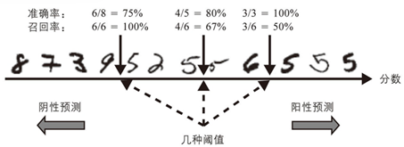
准确率召回率权衡:图像按分类器分数排序,高于所选决策阈值的图像被认为是阳性的。阈值越高,召回率越低,但(通常)准确率越高。
Scikit-Learn不允许你直接设置阈值,但可以让你访问用于预测的决策分数。你可以调用它的 decision_function() 方法,而不是调用分类器的 predict() 方法,该方法返回每个实例的分数,然后根据这些分数使用你想要的任何阈值进行预测。
from sklearn.datasets import fetch_openml
from sklearn.linear_model import SGDClassifier
from sklearn.model_selection import cross_val_predict
from sklearn.metrics import precision_score, recall_score
from sklearn.metrics import f1_score

mnist = fetch_openml('mnist_784', as_frame=False)

X, y = mnist.data, mnist.target

X_train, X_test, y_train, y_test = X[:60000], X[60000:], y[:60000], y[60000:]

y_train_5 = (y_train == '5')
y_test_5 = (y_test == '5')

sgd_clf = SGDClassifier(random_state=42)

sgd_clf.fit(X_train, y_train_5)

some_digit = X[0]

y_scores = sgd_clf.decision_function([some_digit])
print(y_scores)
# [2164.22030239]

threshold = 0
y_some_digit_pred = (y_scores > threshold)
print(y_some_digit_pred)
# [ True]
提高阈值
threshold = 3000
y_some_digit_pred = (y_scores > threshold)
print(y_some_digit_pred)
# [ False]
提高了阈值会降低召回率,图像实际上表示一个5,分类器在阈值为0时检测到它,但当阈值增加到3000时错过了它。
首先,使用 cross_val_predict() 函数获取训练集中所有实例的分数,但这次指定要返回决策分数而不是预测:
from sklearn.datasets import fetch_openml
from sklearn.linear_model import SGDClassifier
from sklearn.model_selection import cross_val_predict
from sklearn.metrics import precision_score, recall_score
from sklearn.metrics import f1_score

mnist = fetch_openml('mnist_784', as_frame=False)

X, y = mnist.data, mnist.target

X_train, X_test, y_train, y_test = X[:60000], X[60000:], y[:60000], y[60000:]

y_train_5 = (y_train == '5')
y_test_5 = (y_test == '5')

sgd_clf = SGDClassifier(random_state=42)

sgd_clf.fit(X_train, y_train_5)

some_digit = X[0]

y_scores = sgd_clf.decision_function([some_digit])

y_scores = cross_val_predict(sgd_clf, X_train, y_train_5, cv=3, method="decision_function")
print(y_scores)
# [  1200.93051237 -26883.79202424 -33072.03475406 ...  13272.12718981
#   -7258.47203373 -16877.50840447]
有了这些分数,使用 precision_recall_curve() 分数计算所有可能的阈值的准确率和召回率(该函数添加最后一个为0的准确率和最后一个为1的召回率,对应于无限阈值):
from sklearn.datasets import fetch_openml
from sklearn.linear_model import SGDClassifier
from sklearn.model_selection import cross_val_predict
from sklearn.metrics import precision_score, recall_score
from sklearn.metrics import f1_score
from sklearn.metrics import precision_recall_curve
import matplotlib.pyplot as plt

mnist = fetch_openml('mnist_784', as_frame=False)

X, y = mnist.data, mnist.target

X_train, X_test, y_train, y_test = X[:60000], X[60000:], y[:60000], y[60000:]

y_train_5 = (y_train == '5')
y_test_5 = (y_test == '5')

sgd_clf = SGDClassifier(random_state=42)

sgd_clf.fit(X_train, y_train_5)

y_scores = cross_val_predict(sgd_clf, X_train, y_train_5, cv=3, method="decision_function")

precisions, recalls, thresholds = precision_recall_curve(y_train_5, y_scores)

plt.plot(thresholds, precisions[:-1], "b--", label="Precision", linewidth=2)
plt.plot(thresholds, recalls[:-1], "g-", label="Recall", linewidth=2)
plt.vlines(thresholds, 0, 1.0, "k", "dotted", label="threshold")

# extra code – this section just beautifies and saves Figure 3–5
idx = (thresholds >= threshold).argmax()  # first index ≥ threshold
plt.plot(thresholds[idx], precisions[idx], "bo")
plt.plot(thresholds[idx], recalls[idx], "go")
plt.axis([-50000, 50000, 0, 1])
plt.grid()
plt.xlabel("Threshold")
plt.legend(loc="center right")

plt.show()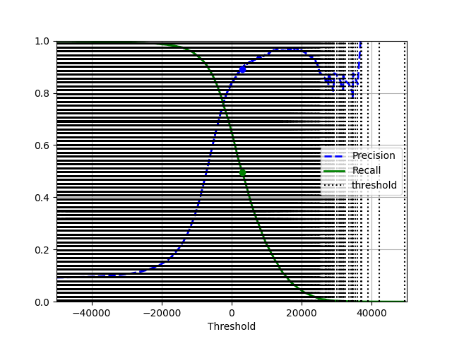
在3000阈值下,准确率接近90%,召回率约为50%。
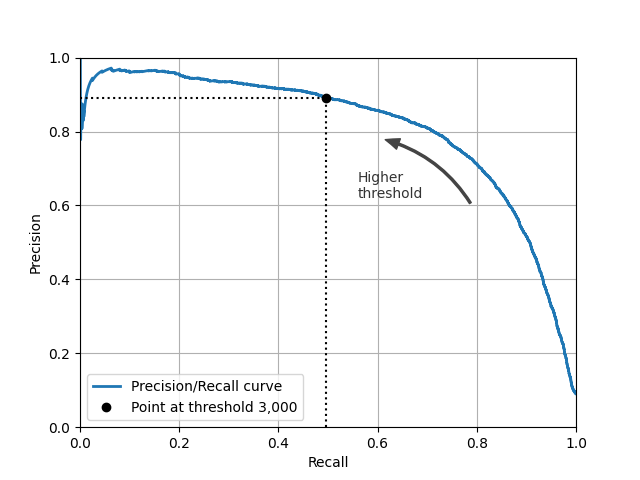
选择一个好的准确率 召回率权衡的另一种方法是直接绘制准确率与召回率的关系图。
from sklearn.datasets import fetch_openml
from sklearn.linear_model import SGDClassifier
from sklearn.model_selection import cross_val_predict
from sklearn.metrics import precision_score, recall_score
from sklearn.metrics import f1_score
from sklearn.metrics import precision_recall_curve
import matplotlib.pyplot as plt
import matplotlib.patches as patches

mnist = fetch_openml('mnist_784', as_frame=False)

X, y = mnist.data, mnist.target

X_train, X_test, y_train, y_test = X[:60000], X[60000:], y[:60000], y[60000:]

y_train_5 = (y_train == '5')
y_test_5 = (y_test == '5')

sgd_clf = SGDClassifier(random_state=42)

sgd_clf.fit(X_train, y_train_5)

y_scores = cross_val_predict(sgd_clf, X_train, y_train_5, cv=3, method="decision_function")

precisions, recalls, thresholds = precision_recall_curve(y_train_5, y_scores)

plt.plot(recalls, precisions, linewidth=2, label="Precision/Recall curve")

idx = (thresholds >= 3000).argmax()
plt.plot([recalls[idx], recalls[idx]], [0., precisions[idx]], "k:")
plt.plot([0.0, recalls[idx]], [precisions[idx], precisions[idx]], "k:")
plt.plot([recalls[idx]], [precisions[idx]], "ko",
         label="Point at threshold 3,000")
plt.gca().add_patch(patches.FancyArrowPatch(
    (0.79, 0.60), (0.61, 0.78),
    connectionstyle="arc3,rad=.2",
    arrowstyle="Simple, tail_width=1.5, head_width=8, head_length=10",
    color="#444444"))
plt.text(0.56, 0.62, "Higher\nthreshold", color="#333333")
plt.xlabel("Recall")
plt.ylabel("Precision")
plt.axis([0, 1, 0, 1])
plt.grid()
plt.legend(loc="lower left")

plt.show()
假设你决定以90%的准确率为目标。可以使用图来找到你需要使用的阈值,但这个不是很准确。或者,你可以搜索为你提供至少90%准确率的最低阈值。
from sklearn.datasets import fetch_openml
from sklearn.linear_model import SGDClassifier
from sklearn.model_selection import cross_val_predict
from sklearn.metrics import precision_score, recall_score
from sklearn.metrics import precision_recall_curve

mnist = fetch_openml('mnist_784', as_frame=False)

X, y = mnist.data, mnist.target

X_train, X_test, y_train, y_test = X[:60000], X[60000:], y[:60000], y[60000:]

y_train_5 = (y_train == '5')
y_test_5 = (y_test == '5')

sgd_clf = SGDClassifier(random_state=42)

sgd_clf.fit(X_train, y_train_5)

y_scores = cross_val_predict(sgd_clf, X_train, y_train_5, cv=3, method="decision_function")

precisions, recalls, thresholds = precision_recall_curve(y_train_5, y_scores)

idx_for_90_precision = (precisions >= 0.90).argmax()
thresholds_for_90_precision = thresholds[idx_for_90_precision]
print(thresholds_for_90_precision)
# 3370.0194991439557

y_train_pred_90 = (y_scores >= thresholds_for_90_precision)
# 检查这个阈值的准确率和召回率
print(precision_score(y_train_5, y_train_pred_90))
# 0.9000345901072293

recall_at_90_precision = recall_score(y_train_5, y_train_pred_90)
print(recall_at_90_precision)
# 0.4799852425751706
太好了,你有一个90%准确率的分类器!如你所见,创建具有你想要的几乎任何准确率的分类器相当容易:只需要设置足够高的阈值。但是等等,不要那么快 如果召回率太低,高准确率分类器就不是很有用!对于许多应用来说,48%的召回率根本算不了什么。
如果有人说:“让我们达到99%的准确率。” 你就应该问:“召回率是多少?”