https://github.com/ageron/handson-ml3/blob/main/02_end_to_end_machine_learning_project.ipynb
什么是端到端机器学习?🤔
端到端机器学习(End-to-End Machine Learning) 是指在一个机器学习项目中,整个流程从数据收集、预处理、模型训练到最终预测结果的输出都由同一个系统或过程自动化完成,且通常是一个整体性的解决方案。简单来说,它就是将各个步骤(如特征工程、模型选择、训练、调优等)整合成一个统一的系统,减少人工干预。
这种方法的优点是能够简化工作流程,提高效率。尤其在深度学习中,端到端模型往往能够直接从原始数据中学习到有用的特征,而不需要人工进行繁琐的特征工程。
举个例子:
假设你想训练一个自动驾驶的系统:
端到端机器学习的典型应用领域有:
这种方法能够减少很多手动的中间环节,但它也要求系统能够处理数据的复杂性和大量的计算。
流行的开放数据存储库
我们将使用来自StatLib存储库的加州房价数据,数据集基于1990年加州人口普查的数据。
回归问题的典型性能度量是均方根误差(Root Mean Square Error,RMSE)。
例如,如果第一个地区如前所述,则矩阵X如下所示:
例如,如果系统预测第一区的房价中位数为158400美元,则
该地区的预测误差为
RMSE(X,h)是使用假设h在样例集上测量的代价函数。
虽然RMSE通常是回归任务的首选性能度量,但在某些情况下,你可能更喜欢使用其他函数。例如,假设有很多异常地区。在这种情况下,你可以考虑使用平均绝对误差(Mean Absolute Error,MAE,也称为平均绝对偏差)
RMSE和MAE都是衡量两个向量(预测向量和目标向量)之间距离的方法。各种距离度量或范数是可能的:
一般而言,包含n个元素的向量v的ℓk范数定义为
ℓ0给出向量中的非零元素的数量,ℓ∞给出向量中的最大绝对值。
范数指数越高,它就越关注大值而忽略小值。这就是RMSE比MAE对异常值更敏感的原因。但是当异常值呈指数级减少时(例如在钟形曲线中),RMSE表现非常好,并且通常是首选。
假设检验是机器学习中一种重要的统计方法,用于评估模型性能、比较不同模型之间的差异,或验证模型假设是否成立。
假设检验在机器学习中主要有以下几个用途:
根据具体问题和数据特性,机器学习中常用的假设检验方法包括:
假设检验通常按照以下步骤进行:
假设检验在机器学习中有多种实际应用场景:
在使用假设检验时,需要关注以下几点:
背景
假设你是一个健身教练,有两种不同的减肥方法:方法A(每天跑步30分钟)和方法B(每天跳绳30分钟)。你想知道这两种方法哪一种对减肥更有效。为了验证效果,你找了20个朋友参与实验,随机分成两组:
一个月后,你记录了每组朋友的体重减少情况,结果如下:
目标
你想知道:
方法B是否真的比方法A更有效?
还是这0.5公斤的差异只是巧合?
用假设检验来解决问题
假设检验是一个科学的工具,可以帮助我们判断这种差异是不是偶然的。以下是具体步骤:
提出假设:
选择检验方法:
因为我们比较的是两组的平均减重,而且样本量较小(每组10人),可以用t-检验来分析。
计算p值:
用统计公式(这里略去复杂计算)分析两组数据:方法A平均减重2公斤,方法B平均减重2.5公斤。 假设计算后得到的p值为0.03。
做出决策:
我们设定一个标准(显著性水平),比如0.05(这是常用的门槛)。
如果p值 < 0.05,就认为差异不是偶然的,拒绝零假设。
这里p值是0.03,小于0.05,所以我们拒绝零假设。
结论
结果:方法B(平均减重2.5公斤)比方法A(平均减重2公斤)的减肥效果显著更好,0.5公斤的差异不是偶然发生的。
通俗解释:
零假设就像在说:“两种方法效果差不多,0.5公斤的差距只是运气。”
p值0.03的意思是:“如果两种方法真的一样好,我们看到这种差距的概率只有3%,很小,所以不太可能是运气。”
因为3% < 5%,我们有信心说方法B确实更有效。
现实意义
根据这个结果,你可以向客户推荐每天跳绳30分钟(方法B),因为数据表明它比跑步更有效。这种方法还能用在其他场景,比如比较两种学习方法、两种广告策略,甚至两种药物的效果。
https://github.com/ageron/data/blob/main/housing/housing.csv
head() 方法查看前5行数据
import pandas as pd

housing = pd.read_csv("housing.csv")

print(housing.head())每一行代表一个地区。有10个属性:longitude、latitude、housing_median_age、total_rooms、total_bedrooms、population、households、median_income、median_house_value和ocean_proximity。
   longitude  latitude  housing_median_age  ...  median_income  median_house_value  ocean_proximity
0    -122.23     37.88                41.0  ...         8.3252            452600.0         NEAR BAY
1    -122.22     37.86                21.0  ...         8.3014            358500.0         NEAR BAY
2    -122.24     37.85                52.0  ...         7.2574            352100.0         NEAR BAY
3    -122.25     37.85                52.0  ...         5.6431            341300.0         NEAR BAY
4    -122.25     37.85                52.0  ...         3.8462            342200.0         NEAR BAY

[5 rows x 10 columns]
info()方法对于获取数据的快速描述很有用,特别是总行数、每个属性的类型和非空值的数量:
housing.info()<class 'pandas.core.frame.DataFrame'>
RangeIndex: 20640 entries, 0 to 20639
Data columns (total 10 columns):
# Column Non-Null Count Dtype
--- ------ -------------- -----
0 longitude 20640 non-null float64
1 latitude 20640 non-null float64
2 housing_median_age 20640 non-null float64
3 total_rooms 20640 non-null float64
4 total_bedrooms 20433 non-null float64
5 population 20640 non-null float64
6 households 20640 non-null float64
7 median_income 20640 non-null float64
8 median_house_value 20640 non-null float64
9 ocean_proximity 20640 non-null object
dtypes: float64(9), object(1)
memory usage: 1.6+ MB使用value_counts()方法找出存在哪些类别以及每个类别有多少个
print(housing["ocean_proximity"].value_counts())ocean_proximity
<1H OCEAN 9136
INLAND 6551
NEAR OCEAN 2658
NEAR BAY 2290
ISLAND 5
Name: count, dtype: int64describe()方法显示数字属性的摘要
print(housing.describe())std: 标准差
longitude latitude housing_median_age ... households median_income median_house_value
count 20640.000000 20640.000000 20640.000000 ... 20640.000000 20640.000000 20640.000000
mean -119.569704 35.631861 28.639486 ... 499.539680 3.870671 206855.816909
std 2.003532 2.135952 12.585558 ... 382.329753 1.899822 115395.615874
min -124.350000 32.540000 1.000000 ... 1.000000 0.499900 14999.000000
25% -121.800000 33.930000 18.000000 ... 280.000000 2.563400 119600.000000
50% -118.490000 34.260000 29.000000 ... 409.000000 3.534800 179700.000000
75% -118.010000 37.710000 37.000000 ... 605.000000 4.743250 264725.000000
max -114.310000 41.950000 52.000000 ... 6082.000000 15.000100 500001.000000
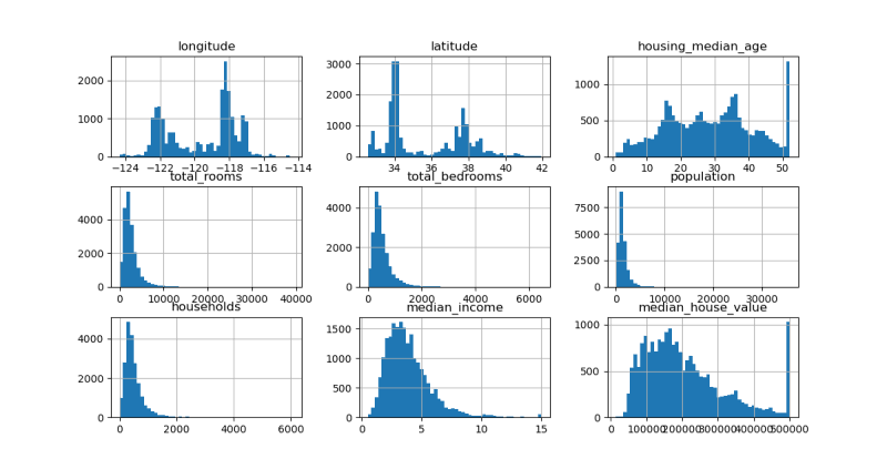
[8 rows x 9 columns]为每个数值属性绘制直方图
import pandas as pd
import matplotlib.pyplot as plt  # 导入 Matplotlib

housing = pd.read_csv("housing.csv")

# bins 决定了直方图中柱子的数量(即数据的分组数量)
# figsize 控制图表的大小(宽度和高度),单位是英寸。
housing.hist(bins=50, figsize=(12, 8))
plt.show()创建测试集在理论上很简单;随机选择一些实例,通常是数据集的20%(如果你的数据集非常大,则更少)
import pandas as pd
import matplotlib.pyplot as plt  # 导入 Matplotlib
import numpy as np

housing = pd.read_csv("housing.csv")

np.random.seed(42)

def shuffle_and_split_data(data, test_ratio):
    shuffled_indices = np.random.permutation(len(data))
    test_set_size = int(len(data) * test_ratio)
    test_indices = shuffled_indices[:test_set_size]
    train_indices = shuffled_indices[test_set_size:]
    print(test_indices) # 打乱分为两组下标
    # [20046  3024 15663 ... 18086  2144  3665]
    print(train_indices)
    # [14196  8267 17445 ...  5390   860 15795]
    return data.iloc[train_indices], data.iloc[test_indices]

print(len(housing))
# 20640

train_set, test_set = shuffle_and_split_data(housing, 0.2)
len(train_set)

print(len(train_set))
# 16512
print(len(test_set))
# 4128为了确保数据划分的可重复性,可以基于数据的标识列(ID)使用哈希函数进行划分。以下代码展示了如何使用 zlib.crc32 函数实现这一功能:
import pandas as pd
import matplotlib.pyplot as plt  # 导入 Matplotlib
import numpy as np
from zlib import crc32

housing = pd.read_csv("housing.csv")

def is_id_in_test_set(identifier, test_ratio):
    return crc32(np.int64(identifier)) < test_ratio * 2**32

def split_data_with_id_hash(data, test_ratio, id_column):
    ids = data[id_column]
    in_test_set = ids.apply(lambda id_: is_id_in_test_set(id_, test_ratio))
    return data.loc[~in_test_set], data.loc[in_test_set]

# 首先为数据集添加索引列(index),然后基于索引列或自定义的 ID 列(通过经纬度计算)进行划分:

print(len(housing))
# 20640

housing_with_id = housing.reset_index()  # adds an `index` column

train_set, test_set = split_data_with_id_hash(housing_with_id, 0.2, "index")

# housing_with_id["id"] = housing["longitude"] * 1000 + housing["latitude"]
# train_set, test_set = split_data_with_id_hash(housing_with_id, 0.2, "id")

len(train_set)

print(len(train_set))
# 16512
print(len(test_set))
# 4128更简单的方法是使用 scikit-learn 的 train_test_split 函数进行随机划分:
import pandas as pd
import matplotlib.pyplot as plt
from sklearn.model_selection import train_test_split

housing = pd.read_csv("housing.csv")

print(len(housing))
# 20640

train_set, test_set = train_test_split(housing, test_size=0.2, random_state=42)

print(len(train_set))
# 16512
print(len(test_set))
# 4128

# 检查缺失值

print(test_set["total_bedrooms"].isnull().sum())
# 44
在测试集中,total_bedrooms 列有 44 个缺失值:
我们已经考虑了纯随机的采样方法。如果你的数据集足够大(尤其是相对于属性的数量),那么这通常没问题。但如果不够大,你就有引入显著采样偏差的风险。当一家调查公司的员工决定打电话给1000个人问他们几个问题时,他们不会只是在电话簿中随机挑选1000个人。就他们想问的问题而言,他们试图确保这1000人代表全体人口。例如,美国人口中女性占51.1%,男性占48.9%,因此在美国进行一项良好的调查需要尝试在样本中保持这一比例:511名女性和489名男性(至少在答案可能因性别而异的情况下)。这称为分层采样:将总体分为称为层的同质子组,并从每个层中抽取正确数量的实例以保证测试集能代表总体。如果进行调查的人使用纯随机采样,则大约有10.7%的机会会抽取到女性参与者少于48.5%或超过53.5%的偏差测试集。无论采用哪种方式,调查结果都可能偏差非常大。
你想计算一个随机抽样(样本量为1000人)中女性比例偏离总体女性比例(51.1%)太多的概率,具体是女性比例低于48.5%或高于53.5%的概率。这是一个统计问题,涉及二项分布,因为抽样中每个个体可以看作是“女性”或“非女性”的二元结果。
二项分布适用于以下场景:
我们需要计算样本中女性人数(成功次数)落在特定范围之外的概率,即女性人数少于485(48.5%)或多于535(53.5%)。
使用 scipy.stats.binom 提供的 cdf()
方法计算累计概率。
from scipy.stats import binom
# 样本数量 1000
sample_size = 1000
# 定义总体女性比例
ratio_female = 0.511
# 创建一个二项分布对象 1000试验次数 每次成功概率0.511
# .cdf(x)计算累积分布函数(Cumulative Distribution Function),表示随机变量≤x的概率。
proba_too_small = binom(sample_size, ratio_female).cdf(485 - 1)
proba_too_large = 1 - binom(sample_size, ratio_female).cdf(535)
print(proba_too_small + proba_too_large)
# 输出:0.10736798530929946通过生成大量随机样本,统计满足条件的样本比例来估计概率:
import pandas as pd
import matplotlib.pyplot as plt
import numpy as np  # 导入 NumPy 库

np.random.seed(42)
sample_size = 1000
ratio_female = 0.511
# 100000次抽样
# 每次抽1000个
# 生成一个形状为 (100,000, 1000) 的二维数组,数组中的每个元素是 [0, 1) 区间内的均匀分布随机数。
samples = (np.random.rand(100_000, sample_size) < ratio_female).sum(axis=1)
print(((samples < 485) | (samples > 535)).mean())
# 0.1071为了更好地分析数据分布,将 median_income 列分层为5个收入类型:
import pandas as pd
import matplotlib.pyplot as plt  # 导入 Matplotlib
import numpy as np

housing = pd.read_csv("housing.csv")

# (0, 1.5] (1.5, 3.0] (3.0, 4.5] (4.5, 6.0] (6.0, ∞)
housing["income_cat"] = pd.cut(housing["median_income"],
                               bins=[0., 1.5, 3.0, 4.5, 6., np.inf],
                               labels=[1, 2, 3, 4, 5])

# 生成一个柱状图,显示每个收入类别的频率。
housing["income_cat"].value_counts().sort_index().plot.bar(rot=0, grid=True)

plt.xlabel("Income category")
plt.ylabel("Number of districts")
plt.show()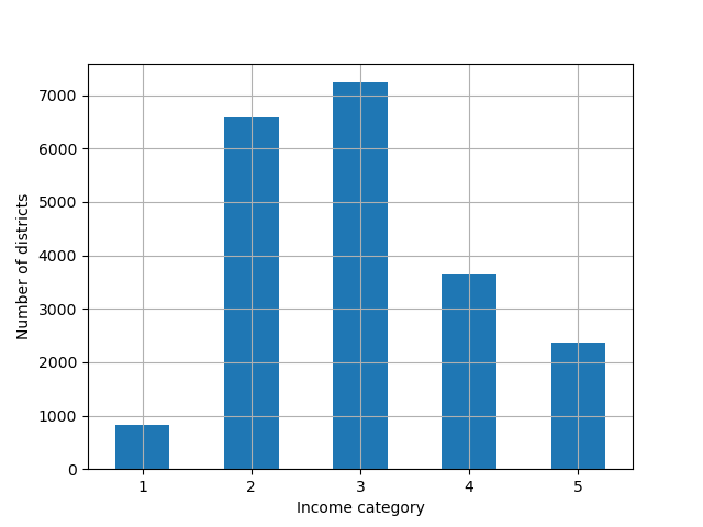
为了确保训练集和测试机地收入类型分布与总体一致,使用
StratifiedShuffleSplit 进行分层抽样:
# 导入必要的库
from sklearn.model_selection import StratifiedShuffleSplit  # 用于分层随机分割数据集
import pandas as pd  # 用于数据处理
import matplotlib.pyplot as plt  # 用于数据可视化
import numpy as np  # 用于数值计算
from sklearn.model_selection import train_test_split  # 用于简单的数据集分割

# 步骤 1:加载数据集
# 从 'housing.csv' 文件中读取住房数据,存储为 pandas DataFrame
housing = pd.read_csv("housing.csv")

# 步骤 2:创建收入类别
# 根据 'median_income' 列,将连续收入值分箱为 5 个类别 (1, 2, 3, 4, 5)
# 分箱区间为 (0, 1.5], (1.5, 3.0], (3.0, 4.5], (4.5, 6.0], (6.0, ∞)
housing["income_cat"] = pd.cut(housing["median_income"],
                               bins=[0., 1.5, 3.0, 4.5, 6., np.inf],
                               labels=[1, 2, 3, 4, 5])

# 步骤 3:使用 StratifiedShuffleSplit 进行分层抽样
# 初始化分层随机分割器,设置 10 次分割,测试集占 20%,随机种子为 42
splitter = StratifiedShuffleSplit(n_splits=10, test_size=0.2, random_state=42)

# 创建一个列表,用于存储每次分割的训练集和测试集
strat_splits = []

# 遍历分割器生成的每次分割的训练和测试索引
for train_index, test_index in splitter.split(housing, housing["income_cat"]):
    # 根据索引提取训练集和测试集
    strat_train_set_n = housing.iloc[train_index]  # 训练集
    strat_test_set_n = housing.iloc[test_index]    # 测试集
    # 将本次分割的训练集和测试集添加到列表
    strat_splits.append([strat_train_set_n, strat_test_set_n])

# 步骤 4:选择第一次分割的训练集和测试集
strat_train_set, strat_test_set = strat_splits[0]

# 步骤 5:打印训练集和测试集的大小
print(len(strat_train_set))  # 输出训练集行数,预期为 16512
print(len(strat_test_set))   # 输出测试集行数,预期为 4128

# 步骤 6:使用 train_test_split 进行更简洁的分层抽样
# 直接使用 train_test_split,设置测试集占 20%,按 'income_cat' 分层,随机种子为 42
strat_train_set, strat_test_set = train_test_split(
    housing, test_size=0.2, stratify=housing["income_cat"], random_state=42)

# 步骤 7:再次打印训练集和测试集的大小
print(len(strat_train_set))  # 输出训练集行数,预期为 16512
print(len(strat_test_set))   # 输出测试集行数,预期为 4128
查看测试集中收入类型的比列
strat_test_set["income_cat"].value_counts() / len(strat_test_set)
# 输出:
# 3    0.350533
# 2    0.318798
# 4    0.176357
# 5    0.114341
# 1    0.039971
# Name: income_cat, dtype: float64通过比较总体、分层抽样和随机抽样的收入类别比例,评估分层抽样的效果:
from sklearn.model_selection import StratifiedShuffleSplit  # 用于分层随机分割数据集
import pandas as pd  # 用于数据处理
import matplotlib.pyplot as plt  # 用于数据可视化
import numpy as np  # 用于数值计算
from sklearn.model_selection import train_test_split  # 用于简单的数据集分割

housing = pd.read_csv("housing.csv")
housing["income_cat"] = pd.cut(housing["median_income"],
                               bins=[0., 1.5, 3.0, 4.5, 6., np.inf],
                               labels=[1, 2, 3, 4, 5])

train_set, test_set = train_test_split(housing, test_size=0.2, random_state=42)

splitter = StratifiedShuffleSplit(n_splits=10, test_size=0.2, random_state=42)

strat_splits = []
for train_index, test_index in splitter.split(housing, housing["income_cat"]):
    strat_train_set_n = housing.iloc[train_index].copy()
    strat_test_set_n = housing.iloc[test_index].copy()
    strat_splits.append([strat_train_set_n, strat_test_set_n])

strat_train_set, strat_test_set = strat_splits[0]

def income_cat_proportions(data):
    return data["income_cat"].value_counts() / len(data)

compare_props = pd.DataFrame({
    "Overall %": income_cat_proportions(housing),
    "Stratified %": income_cat_proportions(strat_test_set),
    "Random %": income_cat_proportions(test_set),
}).sort_index()

compare_props.index.name = "Income Category"
compare_props["Strat. Error %"] = (compare_props["Stratified %"] /
                                   compare_props["Overall %"] - 1)
compare_props["Rand. Error %"] = (compare_props["Random %"] /
                                  compare_props["Overall %"] - 1)
print((compare_props * 100).round(2))

#                  Overall %  Stratified %  Random %  Strat. Error %  Rand. Error %
# Income Category
# 1                     3.98          4.00      4.24            0.36           6.45
# 2                    31.88         31.88     30.74           -0.02          -3.59
# 3                    35.06         35.05     34.52           -0.01          -1.53
# 4                    17.63         17.64     18.41            0.03           4.42
# 5                    11.44         11.43     12.09           -0.08           5.63

for set_ in (strat_train_set, strat_test_set):
    set_.drop("income_cat", axis=1, inplace=True)
分析
经纬度可视化
from sklearn.model_selection import StratifiedShuffleSplit
import pandas as pd
import matplotlib.pyplot as plt
import numpy as np
from sklearn.model_selection import train_test_split

def get_housing_set():
    housing = pd.read_csv("housing.csv")
    housing["income_cat"] = pd.cut(housing["median_income"],
                                   bins=[0., 1.5, 3.0, 4.5, 6., np.inf],
                                   labels=[1, 2, 3, 4, 5])

    splitter = StratifiedShuffleSplit(n_splits=10, test_size=0.2, random_state=42)

    strat_splits = []
    for train_index, test_index in splitter.split(housing, housing["income_cat"]):
        strat_train_set_n = housing.iloc[train_index].copy()
        strat_test_set_n = housing.iloc[test_index].copy()
        strat_splits.append([strat_train_set_n, strat_test_set_n])

    strat_train_set, strat_test_set = strat_splits[0]

    for set_ in (strat_train_set, strat_test_set):
        set_.drop("income_cat", axis=1, inplace=True)
    return strat_train_set, strat_test_set

strat_train_set, strat_test_set = get_housing_set()
strat_train_set_copy = strat_train_set.copy()
strat_test_set_copy = strat_test_set.copy()

strat_train_set_copy.plot(kind="scatter", x="longitude", y="latitude", grid=True)
plt.show()

strat_test_set_copy.plot(kind="scatter", x="longitude", y="latitude", grid=True)
plt.show()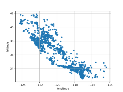
# 房子多的地方颜色更重
strat_train_set_copy.plot(kind="scatter", x="longitude", y="latitude", alpha=0.2)
plt.show()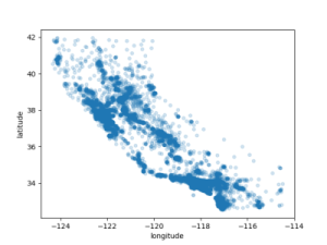
# 根据人口决定图中点的颜色
strat_train_set_copy.plot(kind="scatter", x="longitude", y="latitude", grid=True,
             s=strat_train_set_copy["population"] / 100, label="population",
             c="median_house_value", cmap="jet", colorbar=True,
             legend=True, sharex=False, figsize=(10, 7))
plt.show()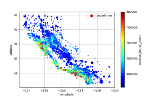
书中作者还搞了个有意思的,以加州地图为画布,把这些点画在加州地图上,可视化效果更加形象。
使用corr()方法计算出每对属性之间的标准相关系数(皮尔逊r)
from sklearn.model_selection import StratifiedShuffleSplit
import pandas as pd
import matplotlib.pyplot as plt
import numpy as np
from sklearn.model_selection import train_test_split

def get_housing():
    return pd.read_csv("housing.csv")

def get_housing_set():
    housing = get_housing()
    housing["income_cat"] = pd.cut(housing["median_income"],
                                   bins=[0., 1.5, 3.0, 4.5, 6., np.inf],
                                   labels=[1, 2, 3, 4, 5])

    splitter = StratifiedShuffleSplit(n_splits=10, test_size=0.2, random_state=42)

    strat_splits = []
    for train_index, test_index in splitter.split(housing, housing["income_cat"]):
        strat_train_set_n = housing.iloc[train_index].copy()
        strat_test_set_n = housing.iloc[test_index].copy()
        strat_splits.append([strat_train_set_n, strat_test_set_n])

    strat_train_set, strat_test_set = strat_splits[0]

    for set_ in (strat_train_set, strat_test_set):
        set_.drop("income_cat", axis=1, inplace=True)
    return strat_train_set, strat_test_set

# strat_train_set, strat_test_set = get_housing_set()
# strat_train_set_copy = strat_train_set.copy()
# strat_test_set_copy = strat_test_set.copy()

housing = get_housing()

print(housing.describe())
#           longitude      latitude  housing_median_age   total_rooms  ...    population    households  median_income  median_house_value
# count  20640.000000  20640.000000        20640.000000  20640.000000  ...  20640.000000  20640.000000   20640.000000        20640.000000
# mean    -119.569704     35.631861           28.639486   2635.763081  ...   1425.476744    499.539680       3.870671       206855.816909
# std        2.003532      2.135952           12.585558   2181.615252  ...   1132.462122    382.329753       1.899822       115395.615874
# min     -124.350000     32.540000            1.000000      2.000000  ...      3.000000      1.000000       0.499900        14999.000000
# 25%     -121.800000     33.930000           18.000000   1447.750000  ...    787.000000    280.000000       2.563400       119600.000000
# 50%     -118.490000     34.260000           29.000000   2127.000000  ...   1166.000000    409.000000       3.534800       179700.000000
# 75%     -118.010000     37.710000           37.000000   3148.000000  ...   1725.000000    605.000000       4.743250       264725.000000
# max     -114.310000     41.950000           52.000000  39320.000000  ...  35682.000000   6082.000000      15.000100       500001.000000

# [8 rows x 9 columns]

# 使用corr()方法计算出每对属性之间的标准相关系数(皮尔逊r)
corr_matrix = housing.corr(numeric_only=True)

print(corr_matrix["median_house_value"].sort_values(ascending=False))
# median_house_value    1.000000
# median_income         0.688075
# total_rooms           0.134153
# housing_median_age    0.105623
# households            0.065843
# total_bedrooms        0.049686
# population           -0.024650
# longitude            -0.045967
# latitude             -0.144160
# Name: median_house_value, dtype: float64

# 相关系数取值范围为-1到1,越接近1表示存在越强的相关性,例如当收入中位数上升时,房价中位数往往会上升
# 当系数接近-1时,表示存在很强的负相关,可以看到纬度和房价中位数之间存在弱的负相关
# 接近于0的系数意味着不存在线性相关
另一种方法是使用pandas的 scatter_maxtrix() 函数,该函数将每个数值属性与其他每个数值属性进行对比,由于现在有11个数值属性, 你将得到11 * 11 = 121 个图表。
from sklearn.model_selection import StratifiedShuffleSplit
import pandas as pd
import matplotlib.pyplot as plt
import numpy as np
from pandas.plotting import scatter_matrix

def get_housing():
    return pd.read_csv("housing.csv")

def get_housing_set():
    housing = get_housing()
    housing["income_cat"] = pd.cut(housing["median_income"],
                                   bins=[0., 1.5, 3.0, 4.5, 6., np.inf],
                                   labels=[1, 2, 3, 4, 5])

    splitter = StratifiedShuffleSplit(n_splits=10, test_size=0.2, random_state=42)

    strat_splits = []
    for train_index, test_index in splitter.split(housing, housing["income_cat"]):
        strat_train_set_n = housing.iloc[train_index].copy()
        strat_test_set_n = housing.iloc[test_index].copy()
        strat_splits.append([strat_train_set_n, strat_test_set_n])

    strat_train_set, strat_test_set = strat_splits[0]

    for set_ in (strat_train_set, strat_test_set):
        set_.drop("income_cat", axis=1, inplace=True)
    return strat_train_set, strat_test_set

# strat_train_set, strat_test_set = get_housing_set()
# strat_train_set_copy = strat_train_set.copy()
# strat_test_set_copy = strat_test_set.copy()

housing = get_housing()

my_attribytes = ["median_house_value", "median_income", "total_rooms", "housing_median_age"]
scatter_matrix(housing[my_attribytes], figsize=(12,8))
plt.show()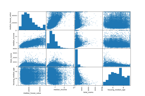
直接用两个属性作坐标值,画散点图
from sklearn.model_selection import StratifiedShuffleSplit
import pandas as pd
import matplotlib.pyplot as plt
from pandas.plotting import scatter_matrix

def get_housing():
    return pd.read_csv("housing.csv")

housing = get_housing()

housing.plot(kind="scatter", x="median_income", y="median_house_value", alpha=0.1, grid=True)
plt.show()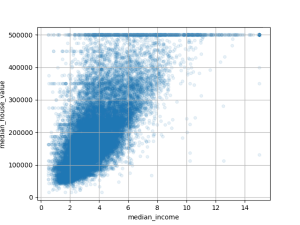
在为机器学习算法准备数据之前,你可能想要做的最后⼀件事是尝试各种属性组合。例如,如 果你不知道⼀个地区有多少户⼈家,则该地区的房间总数就没有多⼤⽤处。你真正想要的是每 个家庭的房间数。同样,卧室总数本身也不是很有⽤:你可能想将其与房间数量进⾏⽐较。每 户⼈⼝似乎也是⼀个值得关注的有趣属性组合。你可以按如下⽅式创建这些新属性:
from sklearn.model_selection import StratifiedShuffleSplit
import pandas as pd
import matplotlib.pyplot as plt
from pandas.plotting import scatter_matrix

def get_housing():
    return pd.read_csv("housing.csv")

housing = get_housing()

# 每个house几个房间
housing["rooms_per_house"] = housing["total_rooms"] / housing["households"]
# 卧室占全部房间的比例
housing["bedrooms_ratio"] = housing["total_bedrooms"] / housing["total_rooms"]
# 一个house几个人
housing["people_per_house"] = housing["population"] / housing["households"]

corr_matrix = housing.corr(numeric_only=True)
print(corr_matrix["median_house_value"].sort_values(ascending=False))

# median_house_value    1.000000
# median_income         0.688075
# rooms_per_house       0.151948
# total_rooms           0.134153
# housing_median_age    0.105623
# households            0.065843
# total_bedrooms        0.049686
# people_per_house     -0.023737
# population           -0.024650
# longitude            -0.045967
# latitude             -0.144160
# bedrooms_ratio       -0.255880
# Name: median_house_value, dtype: float64
新的 bedrooms_ratio 属性与房价中位数的相关性更高,显然,卧室/房间 比例较低的房子往往更贵。
每户房间的数量也⽐⼀个地区的房间总数更具信息量,显然房⼦越⼤,它们就越贵。
这一轮探索不需要很彻底,关键是要从正确的脚步开始并快速获得见解,这将帮助你获得第一个相当不错的原型。但这是⼀个迭代过程:⼀旦你启动并运⾏了⼀个原型,你就可以分析它的输出来获得更多的⻅解并返回到这个探索步骤。
是时候为你的机器学习算法准备数据了,这里你应该为了这个目的编写函数,而不是手动执行此操作,原因如下:
from sklearn.model_selection import StratifiedShuffleSplit
import pandas as pd
import matplotlib.pyplot as plt
import numpy as np
from pandas.plotting import scatter_matrix

def get_housing():
    return pd.read_csv("housing.csv")

def get_housing_set():
    housing = get_housing()
    # 根据median_income进行分层,分为 1 2 3 4 5个等级
    housing["income_cat"] = pd.cut(housing["median_income"],
                                   bins=[0., 1.5, 3.0, 4.5, 6., np.inf],
                                   labels=[1, 2, 3, 4, 5])

    splitter = StratifiedShuffleSplit(n_splits=10, test_size=0.2, random_state=42)

    strat_splits = []
    for train_index, test_index in splitter.split(housing, housing["income_cat"]):
        strat_train_set_n = housing.iloc[train_index].copy()
        strat_test_set_n = housing.iloc[test_index].copy()
        strat_splits.append([strat_train_set_n, strat_test_set_n])

    strat_train_set, strat_test_set = strat_splits[0]

    for set_ in (strat_train_set, strat_test_set):
        set_.drop("income_cat", axis=1, inplace=True)
    return strat_train_set, strat_test_set

strat_train_set, strat_test_set = get_housing_set()

strat_train_set_copy = strat_train_set.copy()
strat_test_set_copy = strat_test_set.copy()

# 将训练数据集的预测变量和标签分开
real_train_set = strat_train_set_copy.drop("median_house_value", axis=1)
real_train_labels = strat_train_set_copy["median_house_value"].copy()

print(real_train_set)
print(real_train_labels)

#        longitude  latitude  housing_median_age  total_rooms  total_bedrooms  population  households  median_income ocean_proximity
# 13096    -122.42     37.80                52.0       3321.0          1115.0      1576.0      1034.0         2.0987        NEAR BAY
# 14973    -118.38     34.14                40.0       1965.0           354.0       666.0       357.0         6.0876       <1H OCEAN
# 3785     -121.98     38.36                33.0       1083.0           217.0       562.0       203.0         2.4330          INLAND
# 14689    -117.11     33.75                17.0       4174.0           851.0      1845.0       780.0         2.2618          INLAND
# 20507    -118.15     33.77                36.0       4366.0          1211.0      1912.0      1172.0         3.5292      NEAR OCEAN
# ...          ...       ...                 ...          ...             ...         ...         ...            ...             ...
# 14207    -118.40     33.86                41.0       2237.0           597.0       938.0       523.0         4.7105       <1H OCEAN
# 13105    -119.31     36.32                23.0       2945.0           592.0      1419.0       532.0         2.5733          INLAND
# 19301    -117.06     32.59                13.0       3920.0           775.0      2814.0       760.0         4.0616      NEAR OCEAN
# 19121    -118.40     34.06                37.0       3781.0           873.0      1725.0       838.0         4.1455       <1H OCEAN
# 19888    -122.41     37.66                44.0        431.0           195.0       682.0       212.0         3.2833      NEAR OCEAN

# [16512 rows x 9 columns]
# 13096    458300.0
# 14973    483800.0
# 3785     101700.0
# 14689     96100.0
# 20507    361800.0
#            ...
# 14207    500001.0
# 13105     88800.0
# 19301    148800.0
# 19121    500001.0
# 19888    233300.0
# Name: median_house_value, Length: 16512, dtype: float64大多数机器学习算法无法处理缺失的特征,因此需要处理。例如,total_bedrooms属性有一些缺失值,可以通过三个选项来解决此问题:
可以用pandas DataFrame的dropna() drop() fillna() 方法完成三种选项
import pandas as pd

def get_housing():
    housing = pd.read_csv("housing.csv")
    return housing

housing = get_housing()

# 输出所有列名
print(housing.columns.tolist())
# ['longitude', 'latitude', 'housing_median_age', 'total_rooms', 'total_bedrooms', 'population', 'households', 'median_income', 'median_house_value', 'ocean_proximity']

for key in housing.columns.tolist():
    print(key, housing[key].isnull().sum(), "/", len(housing[key]))

# longitude 0 / 20640
# latitude 0 / 20640
# housing_median_age 0 / 20640
# total_rooms 0 / 20640
# total_bedrooms 207 / 20640
# population 0 / 20640
# households 0 / 20640
# median_income 0 / 20640
# median_house_value 0 / 20640
# ocean_proximity 0 / 20640

# 可见total_bedrooms有缺失值

# 选项1
# 删除 total_bedrooms 列中包含缺失值(NaN)的行。inplace=True 表示直接修改原始数据框 housing,而不是返回一个新的数据框。
housing_copy1 = housing.copy()
housing_copy1.dropna(subset=["total_bedrooms"], inplace=True)
print(len(housing_copy1)) # 20433

# 选项2
# 删除整个 total_bedrooms 列。axis=1 表示按列操作。执行后,数据框的列数会减少(从 10 列变为 9 列),行数保持不变(20640 行)。
# 注意,此操作不修改原始数据框(需要赋值,如 housing = housing.drop(...) 或添加 inplace=True)。
housing_copy2 = housing.copy()
housing_copy2.drop("total_bedrooms", axis=1, inplace=True)
print(len(housing_copy2.columns.tolist())) # 9
print(("total_bedrooms" in housing_copy2.columns.tolist())) # False

# 选项3
# 用 total_bedrooms 列的中位数填充该列的缺失值。首先计算 total_bedrooms 的中位数
housing_copy3 = housing.copy()
median = housing["total_bedrooms"].median()
print(median) # 435.0
housing_copy3["total_bedrooms"] = housing_copy3["total_bedrooms"].fillna(median)
print(housing_copy3["total_bedrooms"].isnull().sum()) # 0
决定选择选项3,因为它破坏性最小,方便的使用 Scikit-Learn类: SimpleImputer而不是前面的代码。
import pandas as pd
from sklearn.impute import SimpleImputer
import numpy as np

def get_housing():
    housing = pd.read_csv("housing.csv")
    return housing

housing = get_housing()

# 输出所有列名
print(housing.columns.tolist())
# ['longitude', 'latitude', 'housing_median_age', 'total_rooms', 'total_bedrooms', 'population', 'households', 'median_income', 'median_house_value', 'ocean_proximity']

for key in housing.columns.tolist():
    print(key, housing[key].isnull().sum(), "/", len(housing[key]))

# longitude 0 / 20640
# latitude 0 / 20640
# housing_median_age 0 / 20640
# total_rooms 0 / 20640
# total_bedrooms 207 / 20640
# population 0 / 20640
# households 0 / 20640
# median_income 0 / 20640
# median_house_value 0 / 20640
# ocean_proximity 0 / 20640

# 平均值(strategy="mean"),或替换为最频繁的
# 值(strategy="most_frequent"),或替换为常数值(strategy="constant",fill_value=...)。最后两
# 种策略⽀持⾮数值数据。
imputer = SimpleImputer(strategy="median")
# 从 housing 数据框中选择所有数值型列(numeric columns),生成一个新的数据框 housing_num,只包含这些数值型列。
housing_num = housing.select_dtypes(include=[np.number])
print(housing_num)

# 将housing数值型数据拟合到imputer
imputer.fit(housing_num)
print(imputer.statistics_)
# [-1.1849e+02  3.4260e+01  2.9000e+01  2.1270e+03  4.3500e+02  1.1660e+03
#   4.0900e+02  3.5348e+00  1.7970e+05]
print(housing_num.median().values)
# [-1.1849e+02  3.4260e+01  2.9000e+01  2.1270e+03  4.3500e+02  1.1660e+03
#   4.0900e+02  3.5348e+00  1.7970e+05]

# 207
print(housing_num["total_bedrooms"].isnull().sum())
print(imputer.strategy) # median
# imputer处理缺失值
X = imputer.transform(housing_num)
print(len(X))
# 20640
print(len(X[0]))
# 9
print(imputer.feature_names_in_)
# ['longitude' 'latitude' 'housing_median_age' 'total_rooms'
#  'total_bedrooms' 'population' 'households' 'median_income'
#  'median_house_value']


print(housing_num.columns)
# Index(['longitude', 'latitude', 'housing_median_age', 'total_rooms',
#        'total_bedrooms', 'population', 'households', 'median_income',
#        'median_house_value'],
#       dtype='object')
print(housing_num.index)
# Index(['longitude', 'latitude', 'housing_median_age', 'total_rooms',
#        'total_bedrooms', 'population', 'households', 'median_income',
#        'median_house_value'],
#       dtype='object')
# RangeIndex(start=0, stop=20640, step=1)
housing_tr = pd.DataFrame(X, columns=housing_num.columns,
                          index=housing_num.index)
print(housing_tr.describe())
#           longitude      latitude  housing_median_age   total_rooms  total_bedrooms    population    households  median_income  median_house_value
# count  20640.000000  20640.000000        20640.000000  20640.000000    20640.000000  20640.000000  20640.000000   20640.000000        20640.000000
# mean    -119.569704     35.631861           28.639486   2635.763081      536.838857   1425.476744    499.539680       3.870671       206855.816909
# std        2.003532      2.135952           12.585558   2181.615252      419.391878   1132.462122    382.329753       1.899822       115395.615874
# min     -124.350000     32.540000            1.000000      2.000000        1.000000      3.000000      1.000000       0.499900        14999.000000
# 25%     -121.800000     33.930000           18.000000   1447.750000      297.000000    787.000000    280.000000       2.563400       119600.000000
# 50%     -118.490000     34.260000           29.000000   2127.000000      435.000000   1166.000000    409.000000       3.534800       179700.000000
# 75%     -118.010000     37.710000           37.000000   3148.000000      643.250000   1725.000000    605.000000       4.743250       264725.000000
# max -114.310000 41.950000 52.000000 39320.000000 6445.000000 35682.000000 6082.000000 15.000100 500001.000000Scikit-Learn的API设计得非常好,这些是主要设计原则:
一致性所有对象共享一个一致且简单得接口
估计器任何可以根据数据集估计某些参数的对象都称为估计器(例如,SimpleImputer是估计器)。估计本身由fit()⽅法执⾏,它将⼀个数据集作为参数(或两个数据集⽤于监督学习算法,第⼆个 数据集包含标签)。指导估计过程所需的任何其他参数都被视为超参数(例如SimpleImputer的strategy),并且必须将其设置为实例变量(通常通过构造函数参数)。
转换器⼀些估计器(例如SimpleImputer)也可以转换数据集,这些被称为转换器。同样,API很简单:转换由transform()⽅法执⾏,将要转换的数据集作为参数。它返回转换后的数据集。这种转 换通常依赖于学习到的参数,就像SimpleImputer的情况⼀样。所有的转换器还有⼀个名为fit_transform()的便捷⽅法,相当于先调⽤fit()再调⽤transform()(但有时fit_transform()会经过优化,运⾏速度更快)。
预测器最后,⼀些估计器在给定数据集的情况下能够进⾏预测,这些被称为预测器。例如,第1章中的LinearRegression模型是⼀个预测器,给定⼀个国家的⼈均GDP,它预测⽣活满意度。预测器 有⼀个predict()⽅法,它获取新实例的数据集并返回相应预测的数据集。它还有⼀个score()⽅法,可以在给定测试集(以及,在监督学习算法中对应的标签)的情况下测量预测的质量 。
检查所有估计器的超参数都可以通过公开实例变量(例如,imputer.strategy)直接访问,并且所有估计器的学习参数可以通过带有下划线后缀的公共实例变量访问(例如,imputer.statistics_)。
防止类扩散数据集表示为NumPy数组或SciPy稀疏矩阵,⽽不是⾃定义类。超参数只是常规的Python字符串或数字。
构成尽可能重⽤现有的构建块。例如,正如你看到的,很容易从任意序列的转换器来创建⼀个Pipeline估计器,然后是最终估计器。
合理的默认值Scikit-Learn为⼤多数参数提供了合理的默认值,可以轻松快速地创建基本⼯作系统。
Scikit-Learn转换器输出NumPy数组(或有时是SciPy稀疏矩阵),即使将Pandas DataFrame 作为输⼊ 。因此,imputer.transform(housing_num)的输出是⼀个 NumPy数组:X既没有列名 也没有索引。幸运的是,将X包装在DataFrame中并从housing_num中恢复列名和索引并不难:
housing_tr = pd.DataFrame(X, columns=housing_num.columns,
index=housing_num.index)目前为止,只处理了数字属性,但是数据可能包含文本属性。在这个数据集中,只有一个 ocean_proximity属性。
import pandas as pd
from sklearn.impute import SimpleImputer
import numpy as np

def get_housing():
    housing = pd.read_csv("housing.csv")
    return housing

housing = get_housing()

# 输出所有列名
print(housing.columns.tolist())
# ['longitude', 'latitude', 'housing_median_age', 'total_rooms', 'total_bedrooms', 'population', 'households', 'median_income', 'median_house_value', 'ocean_proximity']

housing_cat = housing[["ocean_proximity"]]
print(housing_cat.head(8))

#   ocean_proximity
# 0        NEAR BAY
# 1        NEAR BAY
# 2        NEAR BAY
# 3        NEAR BAY
# 4        NEAR BAY
# 5        NEAR BAY
# 6        NEAR BAY
# 7        NEAR BAY
它不是任意文本,可能的值数量有限,每个值代表一个类别。所以这个属性是一个类别属性。大多数机器学习算法更喜欢处理数字,所以让我们将这些类别从文本转换为数字。
import pandas as pd
from sklearn.impute import SimpleImputer
import numpy as np
from sklearn.preprocessing import OrdinalEncoder

def get_housing():
    housing = pd.read_csv("housing.csv")
    return housing

housing = get_housing()

# 输出所有列名
print(housing.columns.tolist())
# ['longitude', 'latitude', 'housing_median_age', 'total_rooms', 'total_bedrooms', 'population', 'households', 'median_income', 'median_house_value', 'ocean_proximity']

housing_cat = housing[["ocean_proximity"]]
print(housing_cat[:800:100])

#     ocean_proximity
# 0          NEAR BAY
# 100       <1H OCEAN
# 200       <1H OCEAN
# 300          INLAND
# 400          INLAND
# 500       <1H OCEAN
# 600          INLAND
# 700       <1H OCEAN

ordinal_encoder = OrdinalEncoder()
housing_cat_encoded = ordinal_encoder.fit_transform(housing_cat)
print(housing_cat_encoded[:800:100])
# [[3.]
#  [0.]
#  [0.]
#  [1.]
#  [1.]
#  [0.]
#  [1.]
#  [0.]]

# 可以使用categories实例变量来获取类别列表,它是一个包含每个分类属性的一维类别数组的列表,本实例中,列表中
# 包含一个数组,因为只有一个分类属性

print(ordinal_encoder.categories_)
# [array(['<1H OCEAN', 'INLAND', 'ISLAND', 'NEAR BAY', 'NEAR OCEAN'],
#       dtype=object)]
这种表示的一个问题是ML算法会假设两个距离较近的值比距离较远的值更相似,这在某些情况下可能没问题,但是
ocean_proximity列明显不是(例如,类别0和4显然比类别0和1更相似)。要解决此问题,常见的解决方案是为每个类创建一个二进制属性:
当类别为 <1H OCEAN 时 这个属性等于1否则为0,当类别为
INLAND时为1否则为0,以此类推,这称为独热编码,只有一个属性会等于1(热),
而其他属性为0(冷)。可以使用 Scikit-Learn
提供的一个OneHotEncoder类来将类别值转为独热向量。
import pandas as pd
from sklearn.preprocessing import OrdinalEncoder
from sklearn.preprocessing import OneHotEncoder

def get_housing():
    housing = pd.read_csv("housing.csv")
    return housing

housing = get_housing()

# 输出所有列名
print(housing.columns.tolist())
# ['longitude', 'latitude', 'housing_median_age', 'total_rooms', 'total_bedrooms', 'population', 'households', 'median_income', 'median_house_value', 'ocean_proximity']

housing_cat = housing[["ocean_proximity"]]
print(housing_cat[:800:100])

#     ocean_proximity
# 0          NEAR BAY
# 100       <1H OCEAN
# 200       <1H OCEAN
# 300          INLAND
# 400          INLAND
# 500       <1H OCEAN
# 600          INLAND
# 700       <1H OCEAN

onehot_encoder = OneHotEncoder(sparse_output=True)
housing_cat_hot = onehot_encoder.fit_transform(housing_cat)
# 默认情况 OneHotEncoder返回的时SciPy系数矩阵不是NumPy数组
# OneHotEncoder传入sparse_output=False则会返回NumPy数组
print(housing_cat_hot.toarray())
# [[0. 0. 0. 1. 0.]
#  [0. 0. 0. 1. 0.]
#  [0. 0. 0. 1. 0.]
#  ...
#  [0. 1. 0. 0. 0.]
#  [0. 1. 0. 0. 0.]
#  [0. 1. 0. 0. 0.]]
print(len(housing_cat_hot.toarray()))
# 20640
print(housing_cat_hot.toarray()[:800:100])
# [[0. 0. 0. 1. 0.]
#  [1. 0. 0. 0. 0.]
#  [1. 0. 0. 0. 0.]
#  [0. 1. 0. 0. 0.]
#  [0. 1. 0. 0. 0.]
#  [1. 0. 0. 0. 0.]
#  [0. 1. 0. 0. 0.]
#  [1. 0. 0. 0. 0.]]
print(onehot_encoder.categories_)
# [array(['<1H OCEAN', 'INLAND', 'ISLAND', 'NEAR BAY', 'NEAR OCEAN'],
#       dtype=object)]
Pandas有一个名为 get_dummies() 的函数,它将每个分类特征转换为独热表示,每个类别有一个二元特征。
import pandas as pd

df_test = pd.DataFrame({"ocean_proximity": ["INLAND", "NEAR BAY"]})
print(df_test)
#   ocean_proximity
# 0          INLAND
# 1        NEAR BAY
print(pd.get_dummies(df_test))
#    ocean_proximity_INLAND  ocean_proximity_NEAR BAY
# 0                    True                     False
# 1                   False                      True
看起来漂亮又简单,为什么不使用它来代替OneHotEncoder呢?OneHotEncoder的优势在于它会记住经过了那些类别的训练。这非常重要,因为一旦 你的模型投入生产,它应该被提供与训练期间完全相同的特征。
import pandas as pd
from sklearn.preprocessing import OrdinalEncoder
from sklearn.preprocessing import OneHotEncoder

def get_housing():
    housing = pd.read_csv("housing.csv")
    return housing

housing = get_housing()

# 输出所有列名
print(housing.columns.tolist())
# ['longitude', 'latitude', 'housing_median_age', 'total_rooms', 'total_bedrooms', 'population', 'households', 'median_income', 'median_house_value', 'ocean_proximity']

housing_cat = housing[["ocean_proximity"]]
print(housing_cat[:800:100])

#     ocean_proximity
# 0          NEAR BAY
# 100       <1H OCEAN
# 200       <1H OCEAN
# 300          INLAND
# 400          INLAND
# 500       <1H OCEAN
# 600          INLAND
# 700       <1H OCEAN

onehot_encoder = OneHotEncoder(sparse_output=True)
housing_cat_hot = onehot_encoder.fit_transform(housing_cat)
# 默认情况 OneHotEncoder返回的时SciPy系数矩阵不是NumPy数组
# OneHotEncoder传入sparse_output=False则会返回NumPy数组
print(housing_cat_hot.toarray())
# [[0. 0. 0. 1. 0.]
#  [0. 0. 0. 1. 0.]
#  [0. 0. 0. 1. 0.]
#  ...
#  [0. 1. 0. 0. 0.]
#  [0. 1. 0. 0. 0.]
#  [0. 1. 0. 0. 0.]]
print(len(housing_cat_hot.toarray()))
# 20640
print(housing_cat_hot.toarray()[:800:100])
# [[0. 0. 0. 1. 0.]
#  [1. 0. 0. 0. 0.]
#  [1. 0. 0. 0. 0.]
#  [0. 1. 0. 0. 0.]
#  [0. 1. 0. 0. 0.]
#  [1. 0. 0. 0. 0.]
#  [0. 1. 0. 0. 0.]
#  [1. 0. 0. 0. 0.]]
print(onehot_encoder.categories_)
# [array(['<1H OCEAN', 'INLAND', 'ISLAND', 'NEAR BAY', 'NEAR OCEAN'],
#       dtype=object)]

df_test = pd.DataFrame({"ocean_proximity": ["INLAND", "NEAR BAY"]})
print(df_test)
#   ocean_proximity
# 0          INLAND
# 1        NEAR BAY
print(pd.get_dummies(df_test))
#    ocean_proximity_INLAND  ocean_proximity_NEAR BAY
# 0                    True                     False
# 1                   False                      True

# 会记忆上面的transform_fit
print(onehot_encoder.transform(df_test).toarray())
# [[0. 1. 0. 0. 0.]
#  [0. 0. 0. 1. 0.]]

df_test_unknow = pd.DataFrame({"ocean_proximity": ["<2H OCEAN", "ISLAND"]})
print(pd.get_dummies(df_test_unknow))
#    ocean_proximity_<2H OCEAN  ocean_proximity_ISLAND
# 0                       True                   False
# 1                      False                    True
# 出现这种情况肯定不太行,不好用
OneHotEncoder更聪明,它会检测未知类别并引发异常。如果你愿意,可以将handle_unknown超 参数设置为“忽略”,在这种情况下,它将只⽤零表示未知类别:
import pandas as pd
from sklearn.preprocessing import OrdinalEncoder
from sklearn.preprocessing import OneHotEncoder

def get_housing():
    housing = pd.read_csv("housing.csv")
    return housing

housing = get_housing()

# 输出所有列名
print(housing.columns.tolist())
# ['longitude', 'latitude', 'housing_median_age', 'total_rooms', 'total_bedrooms', 'population', 'households', 'median_income', 'median_house_value', 'ocean_proximity']

housing_cat = housing[["ocean_proximity"]]
print(housing_cat[:800:100])

#     ocean_proximity
# 0          NEAR BAY
# 100       <1H OCEAN
# 200       <1H OCEAN
# 300          INLAND
# 400          INLAND
# 500       <1H OCEAN
# 600          INLAND
# 700       <1H OCEAN

onehot_encoder = OneHotEncoder(sparse_output=True)
housing_cat_hot = onehot_encoder.fit_transform(housing_cat)
# 默认情况 OneHotEncoder返回的时SciPy系数矩阵不是NumPy数组
# OneHotEncoder传入sparse_output=False则会返回NumPy数组
print(housing_cat_hot.toarray())
# [[0. 0. 0. 1. 0.]
#  [0. 0. 0. 1. 0.]
#  [0. 0. 0. 1. 0.]
#  ...
#  [0. 1. 0. 0. 0.]
#  [0. 1. 0. 0. 0.]
#  [0. 1. 0. 0. 0.]]
print(len(housing_cat_hot.toarray()))
# 20640
print(housing_cat_hot.toarray()[:800:100])
# [[0. 0. 0. 1. 0.]
#  [1. 0. 0. 0. 0.]
#  [1. 0. 0. 0. 0.]
#  [0. 1. 0. 0. 0.]
#  [0. 1. 0. 0. 0.]
#  [1. 0. 0. 0. 0.]
#  [0. 1. 0. 0. 0.]
#  [1. 0. 0. 0. 0.]]
print(onehot_encoder.categories_)
# [array(['<1H OCEAN', 'INLAND', 'ISLAND', 'NEAR BAY', 'NEAR OCEAN'],
#       dtype=object)]

df_test = pd.DataFrame({"ocean_proximity": ["INLAND", "vdfvd"]})
print(df_test)
#   ocean_proximity
# 0          INLAND
# 1           vdfvd

# 此处会抛出异常
try:
    print(onehot_encoder.transform(df_test).toarray())
except ValueError:
    print("抛异常了")
如果你愿意,可以将handle_unknown超参数设置为 ignore,在这种情况下,它将只用零表示未知类别。
# ...... 接着上面代码

# 此处会抛出异常
try:
    print(onehot_encoder.transform(df_test))
except ValueError:
    print("抛异常了")

onehot_encoder.handle_unknown = "ignore"
print(onehot_encoder.transform(df_test).toarray())
# [[0. 1. 0. 0. 0.]
#  [0. 0. 0. 0. 0.]]

# 用全为0表示未知特征值
如果分类属性有大量可能的类别,(例如 国家代码,职业,物种),则独热编码将导致大量输入特征,这可能会减慢训练速度并降低性能。 如果发生这种情况,你可能希望用与类别相关的有用数值特征来替换分类输入,如可以将ocean_proximity特征替换为到海洋的距离。
你也可以使用 https://github.com/scikit-learn-contrib/category_encoders 上的category_encoders包提供的编码器。
或者在处理神经网络时,可以使用称为嵌入的可学习的低维向量替换每个类别。
OneHotEncoder会将fit的特征名记录在 feature_names_in_
属性中,还可以使用方法 get_feature_names_out()
得到文本拼接出的类别名。
import pandas as pd
from sklearn.preprocessing import OrdinalEncoder
from sklearn.preprocessing import OneHotEncoder

def get_housing():
    housing = pd.read_csv("housing.csv")
    return housing

housing = get_housing()

# 输出所有列名
print(housing.columns.tolist())
# ['longitude', 'latitude', 'housing_median_age', 'total_rooms', 'total_bedrooms', 'population', 'households', 'median_income', 'median_house_value', 'ocean_proximity']

housing_cat = housing[["ocean_proximity"]]
print(housing_cat[:800:100])

#     ocean_proximity
# 0          NEAR BAY
# 100       <1H OCEAN
# 200       <1H OCEAN
# 300          INLAND
# 400          INLAND
# 500       <1H OCEAN
# 600          INLAND
# 700       <1H OCEAN

onehot_encoder = OneHotEncoder(sparse_output=True)
housing_cat_hot = onehot_encoder.fit_transform(housing_cat)
# 默认情况 OneHotEncoder返回的时SciPy系数矩阵不是NumPy数组
# OneHotEncoder传入sparse_output=False则会返回NumPy数组
print(housing_cat_hot.toarray())
# [[0. 0. 0. 1. 0.]
#  [0. 0. 0. 1. 0.]
#  [0. 0. 0. 1. 0.]
#  ...
#  [0. 1. 0. 0. 0.]
#  [0. 1. 0. 0. 0.]
#  [0. 1. 0. 0. 0.]]
print(len(housing_cat_hot.toarray()))
# 20640
print(housing_cat_hot.toarray()[:800:100])
# [[0. 0. 0. 1. 0.]
#  [1. 0. 0. 0. 0.]
#  [1. 0. 0. 0. 0.]
#  [0. 1. 0. 0. 0.]
#  [0. 1. 0. 0. 0.]
#  [1. 0. 0. 0. 0.]
#  [0. 1. 0. 0. 0.]
#  [1. 0. 0. 0. 0.]]
print(onehot_encoder.categories_)
# [array(['<1H OCEAN', 'INLAND', 'ISLAND', 'NEAR BAY', 'NEAR OCEAN'],
#       dtype=object)]

df_test = pd.DataFrame({"ocean_proximity": ["INLAND", "vdfvd"]})
print(df_test)
#   ocean_proximity
# 0          INLAND
# 1           vdfvd

# 此处会抛出异常
try:
    print(onehot_encoder.transform(df_test))
except ValueError:
    print("抛异常了")

onehot_encoder.handle_unknown = "ignore"
print(onehot_encoder.transform(df_test).toarray())
# [[0. 1. 0. 0. 0.]
#  [0. 0. 0. 0. 0.]]

# 用全为0表示未知属性

print(onehot_encoder.feature_names_in_)
# ['ocean_proximity']

print(onehot_encoder.get_feature_names_out())
# ['ocean_proximity_<1H OCEAN' 'ocean_proximity_INLAND'
#  'ocean_proximity_ISLAND' 'ocean_proximity_NEAR BAY'
#  'ocean_proximity_NEAR OCEAN']
print(df_test.index)
# RangeIndex(start=0, stop=2, step=1)
df_output = pd.DataFrame(onehot_encoder.transform(df_test).toarray(),
                         columns=onehot_encoder.get_feature_names_out(),
                         index=df_test.index)
print(df_output.to_string())
#    ocean_proximity_<1H OCEAN  ocean_proximity_INLAND  ocean_proximity_ISLAND  ocean_proximity_NEAR BAY  ocean_proximity_NEAR OCEAN
# 0                        0.0                     1.0                     0.0                       0.0                         0.0
# 1 0.0 0.0 0.0 0.0 0.0你需要应用于数据的最重要的转换之一是特征缩放。除了少数例外,机器学习算法在输入数值属性具有非常不同的尺度时表现不佳。房屋数据就是这种情况:房间总数大约在 6~39320之间,而收入中位数仅在 0~15之间。如果不进行任何缩放,大多数模型将偏向于忽略收入中位数并更多地关注于房间的数量。
有两种常用的方法可以使所有属性具有相同的尺度:最小-最大缩放和标准化。
与所有估计器一样,重要的是仅把缩放器拟合到训练数据:永远不要对训练集以外的任何其他对象使用fit()或fit_transform()。一旦你有了一个训练好的缩放器,你就可以用它来transform()任何其他集合,包括验证集、测试集、新数据。虽然训练集将始终缩放到指定范围,如果新数据包含异常值,这些值可能最终会缩放到范围之外。如果你想避免这种情况,只需将clip超参数设置为True。
import pandas as pd
import numpy as np
from sklearn.preprocessing import MinMaxScaler
from sklearn.preprocessing import StandardScaler

def get_housing():
    housing = pd.read_csv("housing.csv")
    return housing

housing = get_housing()

print(housing.columns.to_list())
# ['longitude', 'latitude', 'housing_median_age', 'total_rooms', 'total_bedrooms', 'population', 'households', 'median_income', 'median_house_value', 'ocean_proximity']

housing_num = housing.select_dtypes(include=[np.number])

# MinMaxScaler 归一化
min_max_scaler = MinMaxScaler(feature_range=(-1, 1))
housing_num_min_max_scaled = min_max_scaler.fit_transform(housing_num)
print("housing_num_min_max_scaled", housing_num_min_max_scaled)
# [[-0.57768924  0.13496281  0.56862745 ... -0.95888834  0.07933684
#    0.80453276]
#  [-0.57569721  0.13071201 -0.21568627 ... -0.62604835  0.07605412
#    0.41649313]
#  [-0.57968127  0.12858661  1.         ... -0.94211478 -0.06794389
#    0.39010148]
#  ...
#  [-0.37649402  0.46439957 -0.37254902 ... -0.85791811 -0.83447125
#   -0.6812343 ]
#  [-0.39641434  0.46439957 -0.33333333 ... -0.88554514 -0.8114095
#   -0.71257438]
#  [-0.38047809  0.45164718 -0.41176471 ... -0.82601546 -0.73949325
#   -0.69319302]]

std_scaler = StandardScaler()
housing_num_std_scaled = std_scaler.fit_transform(housing_num)
print("housing_num_std_scaled", housing_num_std_scaled)
# [[-1.32783522  1.05254828  0.98214266 ... -0.97703285  2.34476576
#    2.12963148]
#  [-1.32284391  1.04318455 -0.60701891 ...  1.66996103  2.33223796
#    1.31415614]
#  [-1.33282653  1.03850269  1.85618152 ... -0.84363692  1.7826994
#    1.25869341]
#  ...
#  [-0.8237132   1.77823747 -0.92485123 ... -0.17404163 -1.14259331
#   -0.99274649]
#  [-0.87362627  1.77823747 -0.84539315 ... -0.39375258 -1.05458292
#   -1.05860847]
#  [-0.83369581  1.75014627 -1.00430931 ...  0.07967221 -0.78012947
# -1.01787803]]标准化是不同的:⾸先它减去平均值(因此标准化值的均值为零),然后将结果除以标准差(因此标准化值的标准差等于1)。与最小-最大缩放不同,标准化不会将值限制在特定范围内。但是,标准化受异常值的影响小得多。
例如一个地区的收入中位数等于100,而不是通常的015。最小-最大缩放到01范围会将此异常值映射到1,并将所有为 StandardScaler的转化器用于标准化。
如果你想缩放稀疏矩阵而不先将其转换为密集矩阵,则可以使用 StandardScaler,并将其 with_mean 超参数设置为 False; 它只会将数据除以标准差,而不减去均值(因为这会破坏稀疏性)。
import pandas as pd
import numpy as np
import matplotlib.pyplot as plt

# 定义函数以加载housing.csv数据集
def get_housing():
    # 读取housing.csv文件并返回DataFrame
    housing = pd.read_csv("housing.csv")
    return housing

# 调用get_housing函数,获取数据集
housing = get_housing()

# 打印数据集的所有列名
print(housing.columns.to_list())
# 输出: ['longitude', 'latitude', 'housing_median_age', 'total_rooms', 'total_bedrooms',
#        'population', 'households', 'median_income', 'median_house_value', 'ocean_proximity']

# 选择数据集中的数值型列,存储到housing_num
housing_num = housing.select_dtypes(include=[np.number])

# 创建一个包含两个子图的图形,尺寸为8x3,共享y轴
fig, axs = plt.subplots(1, 2, figsize=(8, 3), sharey=True)
# 绘制第一个子图:人口列的直方图,分为50个bin
housing["population"].hist(ax=axs[0], bins=50)
# 绘制第二个子图:人口对数列的直方图,分为50个bin
housing["population"].apply(np.log).hist(ax=axs[1], bins=50)
# 设置第一个子图的x轴标签为“Population”
axs[0].set_xlabel("Population")
# 设置第二个子图的x轴标签为“Log of population”
axs[1].set_xlabel("Log of population")
# 设置第一个子图的y轴标签为“Number of districts”
axs[0].set_ylabel("Number of districts")
# 显示图形
plt.show()
为什么使用对数变换?
人口数据通常具有右偏分布(少量地区人口极多,大多数地区人口较少)。对数变换可以:
处理重尾特征的另⼀种⽅法是对特征进⾏分桶(bucketizing)。这意味着将其分布分成⼤致相等⼤⼩的桶,并⽤它所属的桶的索引替换每个特征值,就像我们创建income_cat特征时所做的⼀样(尽管我们只将其⽤于分层采样)。
import pandas as pd
import numpy as np
import matplotlib.pyplot as plt

# 定义函数以加载housing.csv数据集
def get_housing():
    # 读取housing.csv文件并返回DataFrame
    housing = pd.read_csv("housing.csv")
    return housing

# 调用get_housing函数,获取数据集
housing = get_housing()

# 打印数据集的所有列名
print(housing.columns.to_list())
# 输出: ['longitude', 'latitude', 'housing_median_age', 'total_rooms', 'total_bedrooms',
#        'population', 'households', 'median_income', 'median_house_value', 'ocean_proximity']

# 选择数据集中的数值型列,存储到housing_num
housing_num = housing.select_dtypes(include=[np.number])

# 计算median_income列的1到99百分位数
# median_income 列的1到99百分位数(percentiles)是指将 median_income 列的数据按升序排列后,分别计算出1%、2%、3%、...、99%的分位点。这些分位点是将数据分成100等份的关键值,用于描述数据的分布位置。

percentiles = [np.percentile(housing["median_income"], p)
               for p in range(1, 100)]
# 使用pd.cut将median_income分箱,基于百分位数,生成1到100的标签
flattened_median_income = pd.cut(housing["median_income"],
                                 bins=[-np.inf] + percentiles + [np.inf],
                                 labels=range(1, 100 + 1))
# 绘制分箱后的median_income的直方图,分为50个bin
flattened_median_income.hist(bins=50)
# 设置x轴标签为“Median income percentile”
plt.xlabel("Median income percentile")
# 设置y轴标签为“Number of districts”
plt.ylabel("Number of districts")
# 显示图形
plt.show()
# 注意:低于第1百分位数的收入被标记为1,高于第99百分位数的收入被标记为100。这就是为什么下面的分布范围从1到100(而不是0到100)。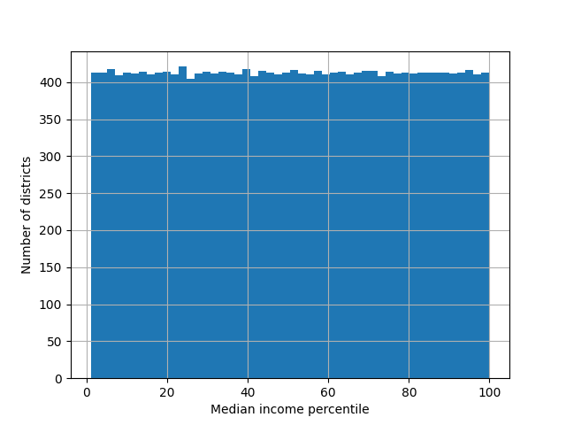
另⼀种转换多峰分布的⽅法是为每个模式(⾄少是主要模式)添加⼀个特征,表示房屋年龄中位数与该特定模式之间的相似性。相似性度量通常使⽤径向基函数 (Radial Basis Function,RBF)计算——任何⼀个仅取决于输⼊值和固定点之间距离的函数。最常⽤的RBF是⾼斯RBF,其输出值随着输⼊值远离固定点⽽呈指数衰减。
例如,房屋年龄x和35之间的⾼斯RBF相似性由⽅程exp(-γ(x-35)2)给出。超参数γ(gamma)决定了当x远离35时相似性度量衰减的速度。
使用Scikit-Learn的rbf_kernel() 函数,可以创建一个新的高斯RBF特征来测量房屋年龄中位数与35之间的相似性。
import pandas as pd
import numpy as np
import matplotlib.pyplot as plt
from sklearn.metrics.pairwise import rbf_kernel

# 定义函数以加载housing.csv数据集
def get_housing():
    # 读取housing.csv文件并返回DataFrame
    housing = pd.read_csv("housing.csv")
    return housing

# 调用get_housing函数,获取数据集
housing = get_housing()

# 打印数据集的所有列名
print(housing.columns.to_list())
# 输出: ['longitude', 'latitude', 'housing_median_age', 'total_rooms', 'total_bedrooms',
#        'population', 'households', 'median_income', 'median_house_value', 'ocean_proximity']

# 选择数据集中的数值型列,存储到housing_num
housing_num = housing.select_dtypes(include=[np.number])

# 使用RBF核计算housing_median_age与年龄35的相似性,gamma=0.1
age_simil_35 = rbf_kernel(housing[["housing_median_age"]], [[35]], gamma=0.1)
# 打印相似性结果
print(age_simil_35)
# 输出示例: [[2.73237224e-02]
#            [3.07487988e-09]
#            [2.81118530e-13]
#            ...
#            [8.48904403e-15]
#            [2.81118530e-13]
#            [2.09879105e-16]]

# 生成从housing_median_age最小值到最大值的500个均匀分布的年龄点
ages = np.linspace(housing["housing_median_age"].min(),
                   housing["housing_median_age"].max(),
                   500).reshape(-1, 1)
# 定义两个gamma值用于RBF核
gamma1 = 0.1
gamma2 = 0.03
# 使用RBF核计算ages与年龄35的相似性,分别使用gamma1和gamma2
rbf1 = rbf_kernel(ages, [[35]], gamma=gamma1)
rbf2 = rbf_kernel(ages, [[35]], gamma=gamma2)

# 创建一个图形和主轴(ax1)
fig, ax1 = plt.subplots()

# 设置主轴的x轴标签为“Housing median age”
ax1.set_xlabel("Housing median age")
# 设置主轴的y轴标签为“Number of districts”
ax1.set_ylabel("Number of districts")
# 绘制housing_median_age的直方图,分为50个bin
ax1.hist(housing["housing_median_age"], bins=50)

# 创建一个共享x轴的副轴(ax2)
ax2 = ax1.twinx()  # create a twin axis that shares the same x-axis
# 设置绘制曲线的颜色
color = "blue"
# 在副轴上绘制gamma=0.1的RBF相似性曲线
ax2.plot(ages, rbf1, color=color, label="gamma = 0.10")
# 在副轴上绘制gamma=0.03的RBF相似性曲线,虚线样式
ax2.plot(ages, rbf2, color=color, label="gamma = 0.03", linestyle="--")
# 设置副轴y轴刻度标签的颜色
ax2.tick_params(axis='y', labelcolor=color)
# 设置副轴的y轴标签为“Age similarity”,颜色与曲线一致
ax2.set_ylabel("Age similarity", color=color)

# 添加图例,位于图形左上角.adobe
plt.legend(loc="upper left")
# 显示图形
plt.show()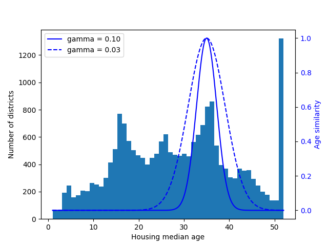
到目前为止,我们只查看了输入特征,但目标值可能还需要转换。训练时转换,那么预测输出值也将会是转换后的值,我们需要转换回去 使用inverse_transform。
import pandas as pd
import matplotlib.pyplot as plt
import numpy as np
from sklearn.model_selection import train_test_split
from sklearn.linear_model import LinearRegression
from sklearn.preprocessing import StandardScaler

# 读取housing.csv数据集
housing = pd.read_csv("housing.csv")

# 根据median_income创建收入类别income_cat,分为5个区间
housing["income_cat"] = pd.cut(housing["median_income"],
                               bins=[0., 1.5, 3.0, 4.5, 6., np.inf],
                               labels=[1, 2, 3, 4, 5])

# 使用分层抽样将数据集分为训练集和测试集,测试集占比20%,按income_cat分层
strat_train_set, strat_test_set = train_test_split(
    housing, test_size=0.2, stratify=housing["income_cat"], random_state=42)

# 打印训练集的行数,预期为16512
print(len(strat_train_set))  # 输出训练集行数
# 打印测试集的行数,预期为4128
print(len(strat_test_set))   # 输出测试集行数

# 从训练集中移除目标列median_house_value,保留特征数据
housing = strat_train_set.drop("median_house_value", axis=1)
# 复制训练集的目标列median_house_value作为标签
housing_labels = strat_train_set["median_house_value"].copy()

# 创建StandardScaler实例,用于对目标值进行特征缩放
target_scaler = StandardScaler()
# 将目标标签转换为DataFrame并进行标准化(均值为0,标准差为1)
scaled_labels = target_scaler.fit_transform(housing_labels.to_frame())
# 创建线性回归模型实例
model = LinearRegression()
# 使用median_income作为特征,训练模型预测缩放后的目标值
model.fit(housing[["median_income"]], scaled_labels)
# 选择训练集中median_income列的前2000行,每200行取一行(共10行)
some_new_data = housing[["median_income"]].iloc[:2000:200]

# 使用模型对some_new_data进行预测,得到缩放后的预测值
scaled_predictions = model.predict(some_new_data)
# 打印缩放后的预测值
print(scaled_predictions)
# 输出示例: [[-0.64466228]
#             [-0.7820197 ]
#             [-0.69341962]
#             [-0.15083051]
#             [-0.67602708]
#             [-0.48347198]
#             [-0.8543916 ]
#             [-0.67489911]
#             [-0.54278128]
#             [ 1.02418492]]

# 使用inverse_transform将缩放后的预测值转换回原始尺度
predictions = target_scaler.inverse_transform(scaled_predictions)
# 打印转换回原始尺度的预测值
print(predictions)
# 输出示例: [[131997.15275877]
#             [116158.39203619]
#             [126374.91716453]
#             [188941.16879238]
#             [128380.46090636]
#             [150584.0958054 ]
#             [107813.14830713]
#             [128510.5275507 ]
#             [143745.10773181]
#             [324432.85091537]]

# 打印训练集中median_house_value列的对应行(前2000行,每200行取一行)
print(strat_train_set[["median_house_value"]].iloc[:2000:200])
# 输出示例:        median_house_value
#            13096            458300.0
#            11916             95500.0
#            3324             186200.0
#            1705             111900.0
#            12357            143000.0
#            19228            125900.0
#            17423             51800.0
#            15452             62800.0
#            867              177900.0
#            20409            500001.0
预测不太准确是正常的,毕竟采用了特征 median_income。单项式。
更简单是的使用 封装好的 TransformedTargetRegressor 帮我们来做上面的事。
import pandas as pd
import matplotlib.pyplot as plt
import numpy as np
from sklearn.model_selection import train_test_split
from sklearn.linear_model import LinearRegression
from sklearn.preprocessing import StandardScaler
from sklearn.compose import TransformedTargetRegressor

housing = pd.read_csv("housing.csv")

housing["income_cat"] = pd.cut(housing["median_income"],
                               bins=[0., 1.5, 3.0, 4.5, 6., np.inf],
                               labels=[1, 2, 3, 4, 5])

strat_train_set, strat_test_set = train_test_split(
    housing, test_size=0.2, stratify=housing["income_cat"], random_state=42)

print(len(strat_train_set))  # 输出训练集行数,预期为 16512
print(len(strat_test_set))   # 输出测试集行数,预期为 4128


housing = strat_train_set.drop("median_house_value", axis=1)
housing_labels = strat_train_set["median_house_value"].copy()


model = TransformedTargetRegressor(LinearRegression(), transformer=StandardScaler())
model.fit(housing[["median_income"]], housing_labels)

some_new_data = housing[["median_income"]].iloc[:2000:200]
predictions = model.predict(some_new_data)
print(pd.DataFrame(predictions))
#                0
# 0  131997.152759
# 1  116158.392036
# 2  126374.917165
# 3  188941.168792
# 4  128380.460906
# 5  150584.095805
# 6  107813.148307
# 7  128510.527551
# 8  143745.107732
# 9  324432.850915
print(strat_train_set[["median_house_value"]].iloc[:2000:200])
#        median_house_value
# 13096            458300.0
# 11916             95500.0
# 3324             186200.0
# 1705             111900.0
# 12357            143000.0
# 19228            125900.0
# 17423             51800.0
# 15452             62800.0
# 867              177900.0
# 20409 500001.0尽管Scikit-Learn提供了许多有用的转换器,但你需要编写自己的转换器来执行自定义转换、清洗操作或组合一些特定的属性等任务。
对于不需要任何训练的转换,只需编写一个函数,将NumPy数组作为输入并输出转换后的数组。
import pandas as pd
import numpy as np
from sklearn.model_selection import train_test_split
from sklearn.preprocessing import FunctionTransformer

housing = pd.read_csv("housing.csv")

housing["income_cat"] = pd.cut(housing["median_income"],
                               bins=[0., 1.5, 3.0, 4.5, 6., np.inf],
                               labels=[1, 2, 3, 4, 5])

strat_train_set, strat_test_set = train_test_split(
    housing, test_size=0.2, stratify=housing["income_cat"], random_state=42)

print(len(strat_train_set))  # 输出训练集行数,预期为 16512
print(len(strat_test_set))   # 输出测试集行数,预期为 4128


housing = strat_train_set.drop("median_house_value", axis=1)
housing_labels = strat_train_set["median_house_value"].copy()

print(housing[["population"]])
#        population
# 13096      1576.0
# 14973       666.0
# 3785        562.0
# 14689      1845.0
# 20507      1912.0
# ...           ...
# 14207       938.0
# 13105      1419.0
# 19301      2814.0
# 19121      1725.0
# 19888       682.0

# [16512 rows x 1 columns]
log_transform = FunctionTransformer(np.log, inverse_func=np.exp)
# inverse_func参数是可选的,它允许你指定一个逆变换函数
log_pop = log_transform.transform(housing[["population"]])
print(log_pop)
#        population
# 13096    7.362645
# 14973    6.501290
# 3785     6.331502
# 14689    7.520235
# 20507    7.555905
# ...           ...
# 14207    6.843750
# 13105    7.257708
# 19301    7.942362
# 19121    7.452982
# 19888 6.525030FunctionTransformer在这段代码中用于对housing数据框的population列进行对数变换。FunctionTransformer
是 sklearn.preprocessing 模块中的一个工具,用于将自定义的
Python 函数(这里是 np.log)转换为与 scikit-learn
流水线和预处理框架兼容的变换器。它允许您对数据应用自定义变换,同时保持与
scikit-learn 生态系统的兼容性。
np.log 指定的变换函数是
np.log,它计算输入数据的自然对数(以 ( e ) 为底)。这里它被应用到
population 列。inverse_func=np.exp:这是一个可选参数,指定了逆变换函数,即指数函数
np.exp。它允许在需要时(例如解释结果或还原数据)将对数变换逆转。虽然这段代码中未使用逆变换,但它在流水线中很有用。housing[["population"]]:输入是一个只包含 population
列的数据框。双括号 [[]] 确保输入是数据框格式,这是
FunctionTransformer 保持列结构的要求。log_pop:
输出是一个数据框,其中population列的值已被转换为它们的自然对数。下面的是将以前的高斯BRF用到FunctionTransformer
import pandas as pd
import numpy as np
from sklearn.model_selection import train_test_split
from sklearn.metrics.pairwise import rbf_kernel
from sklearn.preprocessing import FunctionTransformer

housing = pd.read_csv("housing.csv")

housing["income_cat"] = pd.cut(housing["median_income"],
                               bins=[0., 1.5, 3.0, 4.5, 6., np.inf],
                               labels=[1, 2, 3, 4, 5])

strat_train_set, strat_test_set = train_test_split(
    housing, test_size=0.2, stratify=housing["income_cat"], random_state=42)

print(len(strat_train_set))  # 输出训练集行数,预期为 16512
print(len(strat_test_set))   # 输出测试集行数,预期为 4128


housing = strat_train_set.drop("median_house_value", axis=1)
housing_labels = strat_train_set["median_house_value"].copy()

print(housing[["housing_median_age"]])

rbf_transformer = FunctionTransformer(rbf_kernel, kw_args=dict(Y=[[35.]], gamma=0.1))
age_simil_35 = rbf_transformer.transform(housing[["housing_median_age"]])
print(age_simil_35)
# [[2.81118530e-13]
#  [8.20849986e-02]
#  [6.70320046e-01]
#  ...
#  [9.55316054e-22]
#  [6.70320046e-01]
#  [3.03539138e-04]]
作用:
FunctionTransformer 将 scikit-learn 的 rbf_kernel
函数(径向基函数核)包装为一个变换器,用于计算 housing_median_age
列的值与参考值(这里是 35)的相似性。RBF(径向基函数)核函数的公式表示如下:
Y=[[35.]]下面样例,如何添加一个特征来测量每个地区与旧金山之间的地理相似性:
import pandas as pd
import numpy as np
from sklearn.model_selection import train_test_split
from sklearn.metrics.pairwise import rbf_kernel
from sklearn.preprocessing import FunctionTransformer

housing = pd.read_csv("housing.csv")

housing["income_cat"] = pd.cut(housing["median_income"],
                               bins=[0., 1.5, 3.0, 4.5, 6., np.inf],
                               labels=[1, 2, 3, 4, 5])

strat_train_set, strat_test_set = train_test_split(
    housing, test_size=0.2, stratify=housing["income_cat"], random_state=42)

print(len(strat_train_set))  # 输出训练集行数,预期为 16512
print(len(strat_test_set))   # 输出测试集行数,预期为 4128


housing = strat_train_set.drop("median_house_value", axis=1)
housing_labels = strat_train_set["median_house_value"].copy()

# 旧金山经纬坐标
sf_coords = 37.7749, -122.41
rbf_transformer = FunctionTransformer(rbf_kernel, kw_args=dict(Y=[sf_coords], gamma=0.1))
sf_simil = rbf_transformer.transform(housing[["latitude", "longitude"]])
print(sf_simil)
# [[0.999927  ]
#  [0.05258419]
#  [0.94864161]
#  ...
#  [0.00388525]
#  [0.05038518]
#  [0.99868067]]
自定义转换器也可用于组合特征,例如,有一个计算输入特征0和1之间比率的FunctionTransformer:
import numpy as np
from sklearn.preprocessing import FunctionTransformer

ratio_transformer = FunctionTransformer(lambda X: X[:, [0]] / X[:, [1]])
print(ratio_transformer.transform(np.array([[1., 2.], [3., 4.]])))

# [[0.5 ]
# [0.75]]编一个一个自定义类,类不必继承自任何特定的基类,只需要三个方法,fit() 必须返回self,transform()
和 fit_transform()。
下面有一个与StandardScaler非常相似的自定义转换器。
此实现并没有100%完成:所有估计器在传递DataFrame时都应在fit()⽅法中设
置feature_names_in_。此外,所有的转换器都应该提供⼀个get_feature_names_out()⽅法,以及
⼀个inverse_transform()⽅法,当它们的转换可以被逆转时。:
# 导入必要的基类和工具函数
from sklearn.base import BaseEstimator, TransformerMixin
from sklearn.utils.validation import check_array, check_is_fitted

# 定义自定义标准化类,继承 BaseEstimator 和 TransformerMixin
class StandardScalerClone(BaseEstimator, TransformerMixin):
    # 初始化方法,设置是否减去均值的参数
    def __init__(self, with_mean=True):  # 不使用 *args 或 **kwargs,保持接口简洁
        self.with_mean = with_mean  # 控制是否在标准化时减去均值

    # 拟合方法,计算数据的均值和标准差
    def fit(self, X, y=None):  # y 参数为 scikit-learn 规范要求,尽管未使用
        X = check_array(X)  # 验证 X 为有限浮点数的数组
        self.mean_ = X.mean(axis=0)  # 计算每列均值
        self.scale_ = X.std(axis=0)  # 计算每列标准差
        self.n_features_in_ = X.shape[1]  # 记录输入特征数量(scikit-learn 规范)
        return self  # 返回自身,支持方法链式调用

    # 变换方法,执行标准化(零均值、单位方差)
    def transform(self, X):
        check_is_fitted(self)  # 检查是否已拟合(即是否存在 mean_ 和 scale_ 属性)
        X = check_array(X)  # 验证输入 X 为有效数组
        assert self.n_features_in_ == X.shape[1]  # 确保输入特征数量与拟合时一致
        if self.with_mean:  # 如果 with_mean=True,减去均值
            X = X - self.mean_
        return X / self.scale_  # 除以标准差,完成标准化

# 实例化自定义标准化器
standard_scaler_clone = StandardScalerClone()  # 默认 with_mean=True
自定义转换器可以在其实现中使用其他估计器,如下代码演示了使用KMeans的自定义转换器在fit方法重识别出训练数据中的主要集群,然后在 transform方法中使用 rbf_kernel 测量每个样本与每个集群中心相似程度。
# 导入必要的库
import pandas as pd
import numpy as np
from sklearn.model_selection import train_test_split
from sklearn.metrics.pairwise import rbf_kernel
from sklearn.preprocessing import FunctionTransformer
from sklearn.base import BaseEstimator, TransformerMixin
from sklearn.cluster import KMeans
from sklearn.utils.estimator_checks import check_estimator
# 定义自定义聚类相似性类,继承 BaseEstimator 和 TransformerMixin
class ClusterSimilarity(BaseEstimator, TransformerMixin):
# 初始化方法,设置聚类数、RBF 核参数和随机种子
def __init__(self, n_clusters=10, gamma=1.0, random_state=None):
self.n_clusters = n_clusters # 聚类数量,默认为 10
self.gamma = gamma # RBF 核的宽度参数,默认为 1.0
self.random_state = random_state # 随机种子,确保结果可复现
# 拟合方法,使用 K-Means 聚类数据
def fit(self, X, y=None, sample_weight=None):
# 初始化 K-Means 模型,设置簇数、初始化次数和随机种子
self.kmeans_ = KMeans(self.n_clusters, n_init=10, random_state=self.random_state)
# 拟合 K-Means,sample_weight 允许为数据点分配权重(如房价)
self.kmeans_.fit(X, sample_weight=sample_weight)
return self # 返回自身,支持方法链式调用
# 变换方法,计算输入数据与聚类中心的 RBF 核相似性
def transform(self, X):
# raš rbf_kernel 计算 X 与聚类中心的相似性,gamma 控制宽度
return rbf_kernel(X, self.kmeans_.cluster_centers_, gamma=self.gamma)
# 返回新特征的名称,格式为 "Cluster i similarity"
def get_feature_names_out(self, names=None):
return [f"Cluster {i} similarity" for i in range(self.n_clusters)]
# 加载数据集
housing = pd.read_csv("housing.csv")
# 创建收入分层列,用于分层抽样
housing["income_cat"] = pd.cut(housing["median_income"],
bins=[0., 1.5, 3.0, 4.5, 6., np.inf],
labels=[1, 2, 3, 4, 5])
# 分层拆分数据集,测试集占比 20%,固定随机种子
strat_train_set, strat_test_set = train_test_split(
housing, test_size=0.2, stratify=housing["income_cat"], random_state=42)
# 输出训练集和测试集的行数
print(len(strat_train_set)) # 输出训练集行数,预期为 16512
print(len(strat_test_set)) # 输出测试集行数,预期为 4128
# 从训练集中移除目标变量,保留特征和标签
housing = strat_train_set.drop("median_house_value", axis=1)
housing_labels = strat_train_set["median_house_value"].copy()
# 实例化 ClusterSimilarity,设置 10 个簇、gamma=1.0 和随机种子
cluster_simil = ClusterSimilarity(n_clusters=10, gamma=1., random_state=42)
# 对经纬度数据进行拟合和变换,使用房价作为权重
similarities = cluster_simil.fit_transform(housing[["latitude", "longitude"]],
sample_weight=housing_labels)
# 输出前三行的相似性值,四舍五入到两位小数
print(similarities[:3].round(2))
# [[0.08 0. 0.6 0. 0. 0.99 0. 0. 0. 0.14]
# [0. 0.99 0. 0.04 0. 0. 0.11 0. 0.63 0. ]
# [0.44 0. 0.3 0. 0. 0.7 0. 0.01 0. 0.29]]
# 将实例传给sklearn.utils.estimator_checks包中的check_estimator
# 来检查你的自定义估算器是否遵循Scikit-Learn的API
# print(check_estimator(cluster_simil))
# AssertionError: `ClusterSimilarity.fit()` does not set the `n_features_in_` attribute.
# You might want to use `sklearn.utils.validation.validate_data` instead of `check_array`
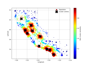
# in `ClusterSimilarity.fit()` which takes care of setting the attribute.下面只用plt展示k均值找到的10个集群中心,这些地区根据其与其最近的集群中心的地理相似性进行着色,如你所见,大多数集群位于人口稠密和昂贵的地区。
import pandas as pd
import numpy as np
from sklearn.model_selection import train_test_split
from sklearn.metrics.pairwise import rbf_kernel
from sklearn.preprocessing import FunctionTransformer
from sklearn.base import BaseEstimator, TransformerMixin
from sklearn.cluster import KMeans
from sklearn.utils.estimator_checks import check_estimator
import matplotlib.pyplot as plt

# 定义自定义聚类相似性类,继承 BaseEstimator 和 TransformerMixin
class ClusterSimilarity(BaseEstimator, TransformerMixin):
    # 初始化方法,设置聚类数、RBF 核参数和随机种子
    def __init__(self, n_clusters=10, gamma=1.0, random_state=None):
        self.n_clusters = n_clusters  # 聚类数量,默认为 10
        self.gamma = gamma  # RBF 核的宽度参数,默认为 1.0
        self.random_state = random_state  # 随机种子,确保结果可复现

    # 拟合方法,使用 K-Means 聚类数据
    def fit(self, X, y=None, sample_weight=None):
        # 初始化 K-Means 模型,设置簇数、初始化次数和随机种子
        self.kmeans_ = KMeans(self.n_clusters, n_init=10, random_state=self.random_state)
        # 拟合 K-Means,sample_weight 允许为数据点分配权重(如房价)
        self.kmeans_.fit(X, sample_weight=sample_weight)
        return self  # 返回自身,支持方法链式调用

    # 变换方法,计算输入数据与聚类中心的 RBF 核相似性
    def transform(self, X):
        # raš rbf_kernel 计算 X 与聚类中心的相似性,gamma 控制宽度
        return rbf_kernel(X, self.kmeans_.cluster_centers_, gamma=self.gamma)

    # 返回新特征的名称,格式为 "Cluster i similarity"
    def get_feature_names_out(self, names=None):
        return [f"Cluster {i} similarity" for i in range(self.n_clusters)]

# 加载数据集
housing = pd.read_csv("housing.csv")

# 创建收入分层列,用于分层抽样
housing["income_cat"] = pd.cut(housing["median_income"],
                               bins=[0., 1.5, 3.0, 4.5, 6., np.inf],
                               labels=[1, 2, 3, 4, 5])

# 分层拆分数据集,测试集占比 20%,固定随机种子
strat_train_set, strat_test_set = train_test_split(
    housing, test_size=0.2, stratify=housing["income_cat"], random_state=42)

# 输出训练集和测试集的行数
print(len(strat_train_set))  # 输出训练集行数,预期为 16512
print(len(strat_test_set))   # 输出测试集行数,预期为 4128

# 从训练集中移除目标变量,保留特征和标签
housing = strat_train_set.drop("median_house_value", axis=1)
housing_labels = strat_train_set["median_house_value"].copy()

# 实例化 ClusterSimilarity,设置 10 个簇、gamma=1.0 和随机种子
cluster_simil = ClusterSimilarity(n_clusters=10, gamma=1., random_state=42)
# 对经纬度数据进行拟合和变换,使用房价作为权重
similarities = cluster_simil.fit_transform(housing[["latitude", "longitude"]],
                                          sample_weight=housing_labels)

# 输出前三行的相似性值,四舍五入到两位小数
print(similarities[:3].round(2))
# [[0.08 0.   0.6  0.   0.   0.99 0.   0.   0.   0.14]
#  [0.   0.99 0.   0.04 0.   0.   0.11 0.   0.63 0.  ]
#  [0.44 0.   0.3  0.   0.   0.7  0.   0.01 0.   0.29]]

# 将实例传给sklearn.utils.estimator_checks包中的check_estimator
# 来检查你的自定义估算器是否遵循Scikit-Learn的API
# print(check_estimator(cluster_simil))
# AssertionError: `ClusterSimilarity.fit()` does not set the `n_features_in_` attribute.
# You might want to use `sklearn.utils.validation.validate_data` instead of `check_array`
# in `ClusterSimilarity.fit()` which takes care of setting the attribute.

# 重命名数据集中的列名,使其更直观
housing_renamed = housing.rename(columns={
    "latitude": "Latitude",  # 将 latitude 重命名为 Latitude
    "longitude": "Longitude",  # 将 longitude 重命名为 Longitude
    "population": "Population",  # 将 population 重命名为 Population
    "median_house_value": "Median house value (ᴜsᴅ)"  # 将 median_house_value 重命名
})

# 添加新列,存储每个数据点与聚类中心的最大相似性
housing_renamed["Max cluster similarity"] = similarities.max(axis=1)

# 绘制散点图,展示地理分布
housing_renamed.plot(kind="scatter", x="Longitude", y="Latitude", grid=True,
                     s=housing_renamed["Population"] / 100, label="Population",  # 散点大小由人口决定
                     c="Max cluster similarity",  # 散点颜色由最大相似性决定
                     cmap="jet", colorbar=True,  # 使用 jet 颜色映射并显示颜色条
                     legend=True, sharex=False, figsize=(10, 7))  # 设置图例、独立 x 轴和图形大小

# 在图上标记 K-Means 聚类中心
plt.plot(cluster_simil.kmeans_.cluster_centers_[:, 1],  # 聚类中心的经度
         cluster_simil.kmeans_.cluster_centers_[:, 0],  # 聚类中心的纬度
         linestyle="", color="black", marker="X", markersize=20,  # 无连线,黑色 X 标记
         label="Cluster centers")  # 图例标签为聚类中心

# 将图例放置在右上角
plt.legend(loc="upper right")

# 显示图形
plt.show()我们需要以正确的顺序执行许多数据转换步骤。Scikit-Learn提供了Pipeline类来帮助处理此类转换序列。下面是一个用于数值属性的小流水线,首先估算然后缩放输入特征。
from sklearn.discriminant_analysis import StandardScaler
from sklearn.impute import SimpleImputer
from sklearn.pipeline import Pipeline, make_pipeline
import sklearn

# 在Jupyter nodebook中,如果你导入sklearn并运行,所有Scikit-Learn估计器都将呈现为交互式图表
# 这对可视化流水线特别有用
sklearn.set_config(display="diagram")

num_pipeline = Pipeline([
    ("impute", SimpleImputer(strategy="median")),
    ("standardize", StandardScaler()),
])

print(num_pipeline)
# Pipeline(steps=[('impute', SimpleImputer(strategy='median')),
#                 ('standardize', StandardScaler())])

# 如果不想给转换器命名,则可以使用make_pipeline函数来替代
num_pipeline_1 = make_pipeline(SimpleImputer(strategy="median"), StandardScaler())
print(num_pipeline_1)
# Pipeline(steps=[('simpleimputer', SimpleImputer(strategy='median')),
#                 ('standardscaler', StandardScaler())])
当你调用流水线的fit()方法时,它会在所有转换器上一次调用fit_transform(),将每次调用的输出作为参数传递给下一次调用,直到它到达最终的估计器,它只调用fit()方法。
如果你调用流水线的transform()方法,它将顺序地将所有转换应用于数据。
如果最后一个估计器是预测器而不是转换器,那么流水线有一个predict() 方法而不是 transform() 方法。调用它会按顺序将所有转换应用于数据并将结果传递给预测器地predict() 方法。
import pandas as pd
import numpy as np
import matplotlib.pyplot as plt
from sklearn.metrics.pairwise import rbf_kernel
from sklearn.discriminant_analysis import StandardScaler
from sklearn.impute import SimpleImputer
from sklearn.pipeline import Pipeline

def get_housing():
    housing = pd.read_csv("housing.csv")
    return housing

housing = get_housing()

print(housing.columns.to_list())
# ['longitude', 'latitude', 'housing_median_age', 'total_rooms', 'total_bedrooms',
#        'population', 'households', 'median_income', 'median_house_value', 'ocean_proximity']

housing_num = housing.select_dtypes(include=[np.number])

num_pipeline = Pipeline([
    ("impute", SimpleImputer(strategy="median")),
    ("standardize", StandardScaler()),
])

# 还能设置参数
num_pipeline.set_params(impute__strategy="median")

housing_num_prepared = num_pipeline.fit_transform(housing_num)
print(housing_num_prepared[:2].round(2))
# [[-1.33  1.05  0.98 -0.8  -0.97 -0.97 -0.98  2.34  2.13]
#  [-1.32  1.04 -0.61  2.05  1.36  0.86  1.67  2.33  1.31]]

# 恢复一个好的DataFrame,可以使用流水线地get_feature_names_out()方法
print(housing_num.index)
# RangeIndex(start=0, stop=20640, step=1)
df_housing_num_prepared = pd.DataFrame(
    housing_num_prepared, columns=num_pipeline.get_feature_names_out(),
    index=housing_num.index
)
print(df_housing_num_prepared.describe())
#           longitude      latitude  housing_median_age   total_rooms  total_bedrooms    population    households  median_income  median_house_value
# count  2.064000e+04  2.064000e+04        2.064000e+04  2.064000e+04    2.064000e+04  2.064000e+04  2.064000e+04   2.064000e+04        2.064000e+04
# mean  -8.556119e-15 -1.046536e-15        3.786807e-17  2.573308e-17   -9.191614e-17 -1.101617e-17  7.435912e-17   5.645785e-17       -9.776848e-17
# std    1.000024e+00  1.000024e+00        1.000024e+00  1.000024e+00    1.000024e+00  1.000024e+00  1.000024e+00   1.000024e+00        1.000024e+00
# min   -2.385992e+00 -1.447568e+00       -2.196180e+00 -1.207283e+00   -1.277688e+00 -1.256123e+00 -1.303984e+00  -1.774299e+00       -1.662641e+00
# 25%   -1.113209e+00 -7.967887e-01       -8.453931e-01 -5.445698e-01   -5.718868e-01 -5.638089e-01 -5.742294e-01  -6.881186e-01       -7.561633e-01
# 50%    5.389137e-01 -6.422871e-01        2.864572e-02 -2.332104e-01   -2.428309e-01 -2.291318e-01 -2.368162e-01  -1.767951e-01       -2.353337e-01
# 75%    7.784964e-01  9.729566e-01        6.643103e-01  2.348028e-01    2.537334e-01  2.644949e-01  2.758427e-01   4.593063e-01        5.014973e-01
# max    2.625280e+00  2.958068e+00        1.856182e+00  1.681558e+01    1.408779e+01  3.025033e+01  1.460152e+01   5.858286e+00        2.540411e+00

print(num_pipeline.steps)
# [('impute', SimpleImputer(strategy='median')), ('standardize', StandardScaler())]
print(num_pipeline[1]) # StandardScaler()
print(num_pipeline[:-1])
# Pipeline(steps=[('impute', SimpleImputer(strategy='median'))])
print(num_pipeline.named_steps["impute"])
# SimpleImputer(strategy='median')
目前为止,我们分别处理了类别列合数值列,拥有一个能够处理所有列的转换器,对每一列适当的转换会更方便。
ColumnTransformer会将num_pipeline应用于数值属性,将cat_pipeline应用于分类属性:
import pandas as pd
import numpy as np
import matplotlib.pyplot as plt
from sklearn.preprocessing import StandardScaler
from sklearn.impute import SimpleImputer
from sklearn.pipeline import Pipeline, make_pipeline
from sklearn.compose import ColumnTransformer
from sklearn.preprocessing import OneHotEncoder
from sklearn.compose import make_column_selector, make_column_transformer

def get_housing():
    housing = pd.read_csv("housing.csv")
    return housing

housing = get_housing()

print(housing.columns.to_list())
# ['longitude', 'latitude', 'housing_median_age', 'total_rooms', 'total_bedrooms',
#        'population', 'households', 'median_income', 'median_house_value', 'ocean_proximity']

num_attribs = ["longitude", "latitude", "housing_median_age", "total_rooms",
               "total_bedrooms", "population", "households", "median_income"]
cat_attribs = ["ocean_proximity"]

num_pipeline = make_pipeline(SimpleImputer(strategy="median"), StandardScaler())

cat_pipeline = make_pipeline(
    SimpleImputer(strategy="most_frequent"),
    OneHotEncoder(handle_unknown="ignore"))

preprocessing_ret = ColumnTransformer([
    ("num", num_pipeline, num_attribs),
    ("cat", cat_pipeline, cat_attribs)
])

# preprocessing = make_column_transformer(
#     (num_pipeline, make_column_selector(dtype_include=np.number)),
#     (cat_pipeline, make_column_selector(dtype_include=object)),
# )

housing_prepared_ret = preprocessing_ret.fit_transform(housing)

housing_prepared_fr = pd.DataFrame(
    housing_prepared_ret,
    columns=preprocessing_ret.get_feature_names_out(),
    index=housing.index)
print(housing_prepared_fr.describe().to_string(max_cols=None))

#        num__longitude  num__latitude  num__housing_median_age  num__total_rooms  num__total_bedrooms  num__population  num__households  num__median_income  cat__ocean_proximity_<1H OCEAN  cat__ocean_proximity_INLAND  cat__ocean_proximity_ISLAND  cat__ocean_proximity_NEAR BAY  cat__ocean_proximity_NEAR OCEAN
# count    2.064000e+04   2.064000e+04             2.064000e+04      2.064000e+04         2.064000e+04     2.064000e+04     2.064000e+04        2.064000e+04                    20640.000000                 20640.000000                 20640.000000                   20640.000000                     20640.000000
# mean    -8.556119e-15  -1.046536e-15             3.786807e-17      2.573308e-17        -9.191614e-17    -1.101617e-17     7.435912e-17        5.645785e-17                        0.442636                     0.317393                     0.000242                       0.110950                         0.128779
# std      1.000024e+00   1.000024e+00             1.000024e+00      1.000024e+00         1.000024e+00     1.000024e+00     1.000024e+00        1.000024e+00                        0.496710                     0.465473                     0.015563                       0.314077                         0.334963
# min     -2.385992e+00  -1.447568e+00            -2.196180e+00     -1.207283e+00        -1.277688e+00    -1.256123e+00    -1.303984e+00       -1.774299e+00                        0.000000                     0.000000                     0.000000                       0.000000                         0.000000
# 25%     -1.113209e+00  -7.967887e-01            -8.453931e-01     -5.445698e-01        -5.718868e-01    -5.638089e-01    -5.742294e-01       -6.881186e-01                        0.000000                     0.000000                     0.000000                       0.000000                         0.000000
# 50%      5.389137e-01  -6.422871e-01             2.864572e-02     -2.332104e-01        -2.428309e-01    -2.291318e-01    -2.368162e-01       -1.767951e-01                        0.000000                     0.000000                     0.000000                       0.000000                         0.000000
# 75%      7.784964e-01   9.729566e-01             6.643103e-01      2.348028e-01         2.537334e-01     2.644949e-01     2.758427e-01        4.593063e-01                        1.000000                     1.000000                     0.000000                       0.000000                         0.000000
# max      2.625280e+00   2.958068e+00             1.856182e+00      1.681558e+01         1.408779e+01     3.025033e+01     1.460152e+01        5.858286e+00                        1.000000                     1.000000                     1.000000                       1.000000                         1.000000
如果使用make_column_transformer则会是下面的情况,列名不一样了
# ...
preprocessing_ret = make_column_transformer(
    (num_pipeline, make_column_selector(dtype_include=np.number)),
    (cat_pipeline, make_column_selector(dtype_include=object)),
)
# ...
print(housing_prepared_fr.describe().to_string(max_cols=None))

# ['longitude', 'latitude', 'housing_median_age', 'total_rooms', 'total_bedrooms', 'population', 'households', 'median_income', 'median_house_value', 'ocean_proximity']
#        pipeline-1__longitude  pipeline-1__latitude  pipeline-1__housing_median_age  pipeline-1__total_rooms  pipeline-1__total_bedrooms  pipeline-1__population  pipeline-1__households  pipeline-1__median_income  pipeline-1__median_house_value  pipeline-2__ocean_proximity_<1H OCEAN  pipeline-2__ocean_proximity_INLAND  pipeline-2__ocean_proximity_ISLAND  pipeline-2__ocean_proximity_NEAR BAY  pipeline-2__ocean_proximity_NEAR OCEAN
# count           2.064000e+04          2.064000e+04                    2.064000e+04             2.064000e+04                2.064000e+04            2.064000e+04            2.064000e+04               2.064000e+04                    2.064000e+04                           20640.000000                        20640.000000                        20640.000000                          20640.000000                            20640.000000
# mean           -8.556119e-15         -1.046536e-15                    3.786807e-17             2.573308e-17               -9.191614e-17           -1.101617e-17            7.435912e-17               5.645785e-17                   -9.776848e-17                               0.442636                            0.317393                            0.000242                              0.110950                                0.128779
# std             1.000024e+00          1.000024e+00                    1.000024e+00             1.000024e+00                1.000024e+00            1.000024e+00            1.000024e+00               1.000024e+00                    1.000024e+00                               0.496710                            0.465473                            0.015563                              0.314077                                0.334963
# min            -2.385992e+00         -1.447568e+00                   -2.196180e+00            -1.207283e+00               -1.277688e+00           -1.256123e+00           -1.303984e+00              -1.774299e+00                   -1.662641e+00                               0.000000                            0.000000                            0.000000                              0.000000                                0.000000
# 25%            -1.113209e+00         -7.967887e-01                   -8.453931e-01            -5.445698e-01               -5.718868e-01           -5.638089e-01           -5.742294e-01              -6.881186e-01                   -7.561633e-01                               0.000000                            0.000000                            0.000000                              0.000000                                0.000000
# 50%             5.389137e-01         -6.422871e-01                    2.864572e-02            -2.332104e-01               -2.428309e-01           -2.291318e-01           -2.368162e-01              -1.767951e-01                   -2.353337e-01                               0.000000                            0.000000                            0.000000                              0.000000                                0.000000
# 75%             7.784964e-01          9.729566e-01                    6.643103e-01             2.348028e-01                2.537334e-01            2.644949e-01            2.758427e-01               4.593063e-01                    5.014973e-01                               1.000000                            1.000000                            0.000000                              0.000000                                0.000000
# max             2.625280e+00          2.958068e+00                    1.856182e+00             1.681558e+01                1.408779e+01            3.025033e+01            1.460152e+01               5.858286e+00                    2.540411e+00                               1.000000                            1.000000                            1.000000                              1.000000                                1.000000
OneHotEncoder返回一个稀疏矩阵,而num_pipeline返回一个密集矩阵。当稀疏矩阵和密集矩阵混合存在时,ColumnTransformer会估计最终矩阵的密度(即非零单元的比率),稀疏阈值默认为
(sparse_threshold=0.3)
我们回顾一下流水线将做什么以及为什么做:
一下将会是我们数据预处理的完整代码,你会发现简单了许多,sklearn帮我们考虑到了这些功能,直接用就好了
import pandas as pd
import numpy as np
import matplotlib.pyplot as plt
from sklearn.preprocessing import StandardScaler
from sklearn.impute import SimpleImputer
from sklearn.pipeline import Pipeline, make_pipeline
from sklearn.compose import ColumnTransformer
from sklearn.preprocessing import OneHotEncoder
from sklearn.compose import make_column_selector, make_column_transformer
from sklearn.preprocessing import FunctionTransformer
from sklearn.cluster import KMeans
from sklearn.metrics.pairwise import rbf_kernel
from sklearn.base import BaseEstimator, TransformerMixin

# 定义函数以加载住房数据集
def get_housing():
    # 读取 housing.csv 文件,返回 DataFrame
    housing = pd.read_csv("housing.csv")
    return housing

# 获取原始住房数据
housing_origin_data = get_housing()

# 删除目标变量 median_house_value,保留特征
housing = housing_origin_data.drop("median_house_value", axis=1)
# 复制目标变量 median_house_value
housing_labels = housing_origin_data["median_house_value"].copy()

# 打印数据集的列名
print(housing.columns.to_list())
# ['longitude', 'latitude', 'housing_median_age', 'total_rooms', 'total_bedrooms',
#  'population', 'households', 'median_income', 'median_house_value', 'ocean_proximity']

# 定义自定义聚类相似性类,继承 BaseEstimator 和 TransformerMixin
class ClusterSimilarity(BaseEstimator, TransformerMixin):
    # 初始化方法,设置聚类数、RBF 核参数和随机种子
    def __init__(self, n_clusters=10, gamma=1.0, random_state=None):
        self.n_clusters = n_clusters  # 聚类数量,默认为 10
        self.gamma = gamma  # RBF 核的宽度参数,默认为 1.0
        self.random_state = random_state  # 随机种子,确保结果可复现

    # 拟合方法,使用 K-Means 聚类数据
    def fit(self, X, y=None, sample_weight=None):
        # 初始化 K-Means 模型,设置簇数、初始化次数和随机种子
        self.kmeans_ = KMeans(self.n_clusters, n_init=10, random_state=self.random_state)
        # 拟合 K-Means,sample_weight 允许为数据点分配权重(如房价)
        self.kmeans_.fit(X, sample_weight=sample_weight)
        return self  # 返回自身,支持方法链式调用

    # 变换方法,计算输入数据与聚类中心的 RBF 核相似性
    def transform(self, X):
        # 使用 rbf_kernel 计算 X 与聚类中心的相似性,gamma 控制宽度
        return rbf_kernel(X, self.kmeans_.cluster_centers_, gamma=self.gamma)

    # 返回新特征的名称,格式为 "Cluster i similarity"
    def get_feature_names_out(self, names=None):
        return [f"Cluster {i} similarity" for i in range(self.n_clusters)]

# 定义计算列比率的函数
def column_ratio(X):
    # 计算第一列与第二列的比率
    return X[:, [0]] / X[:, [1]]

# 定义比率特征的名称
def ratio_name(function_transformer, feature_names_in):
    return ["ratio"]

# 定义比率处理流水线
def ratio_pipeline():
    return make_pipeline(
        SimpleImputer(strategy="median"),  # 用中位数填补缺失值
        FunctionTransformer(column_ratio, feature_names_out=ratio_name),  # 计算比率
        StandardScaler())  # 标准化数据

# 定义对数变换流水线
log_pipeline = make_pipeline(
    SimpleImputer(strategy="median"),  # 用中位数填补缺失值
    FunctionTransformer(np.log, feature_names_out="one-to-one"),  # 应用对数变换
    StandardScaler())  # 标准化数据

# 初始化聚类相似性转换器,设置 10 个簇,gamma=1.0,随机种子为 42
cluster_simil = ClusterSimilarity(n_clusters=10, gamma=1., random_state=42)

# 定义默认数值处理流水线
default_num_pipeline = make_pipeline(
    SimpleImputer(strategy="median"),  # 用中位数填补缺失值
    StandardScaler())  # 标准化数据

# 定义分类变量处理流水线
cat_pipeline = make_pipeline(
    SimpleImputer(strategy="most_frequent"),  # 用众数填补缺失值
    OneHotEncoder(handle_unknown="ignore"))  # 独热编码,忽略未知类别

# 定义预处理 ColumnTransformer,组合多种特征处理方式
preprocessing = ColumnTransformer([
        ("bedrooms", ratio_pipeline(), ["total_bedrooms", "total_rooms"]),  # 卧室/房间比率
        ("rooms_per_house", ratio_pipeline(), ["total_rooms", "households"]),  # 房间/家庭比率
        ("people_per_house", ratio_pipeline(), ["population", "households"]),  # 人口/家庭比率
        ("log", log_pipeline, ["total_bedrooms", "total_rooms", "population",# 对数变换
                               "households", "median_income"]),
        ("geo", cluster_simil, ["latitude", "longitude"]),  # 地理位置聚类相似性
        ("cat", cat_pipeline, make_column_selector(dtype_include=object)),  # 分类变量处理
    ],
    remainder=default_num_pipeline)  # 剩余列(housing_median_age)使用默认流水线

# 应用预处理流水线,转换数据集
housing_prepared = preprocessing.fit_transform(housing)
# 打印转换后数据的形状
print(housing_prepared.shape)
# (20640, 24)

# 打印转换后特征的名称
print(preprocessing.get_feature_names_out())
# ['bedrooms__ratio' 'rooms_per_house__ratio' 'people_per_house__ratio'
#  'log__total_bedrooms' 'log__total_rooms' 'log__population'
#  'log__households' 'log__median_income' 'geo__Cluster 0 similarity'
#  'geo__Cluster 1 similarity' 'geo__Cluster 2 similarity'
#  'geo__Cluster 3 similarity' 'geo__Cluster 4 similarity'
#  'geo__Cluster 5 similarity' 'geo__Cluster 6 similarity'
#  'geo__Cluster 7 similarity' 'geo__Cluster 8 similarity'
#  'geo__Cluster 9 similarity' 'cat__ocean_proximity_<1H OCEAN'
#  'cat__ocean_proximity_INLAND' 'cat__ocean_proximity_ISLAND'
#  'cat__ocean_proximity_NEAR BAY' 'cat__ocean_proximity_NEAR OCEAN'
#  'remainder__housing_median_age']

# 将转换后的数据转换为 DataFrame,保留特征名称和原始索引
housing_prepared_fr = pd.DataFrame(housing_prepared,
                                   columns=preprocessing.get_feature_names_out(),
                                   index=housing.index)
# 打印前两行数据
print(housing_prepared_fr.head(2))
#    bedrooms__ratio  rooms_per_house__ratio  people_per_house__ratio  log__total_bedrooms  log__total_rooms  ...  cat__ocean_proximity_INLAND  cat__ocean_proximity_ISLAND  cat__ocean_proximity_NEAR BAY  cat__ocean_proximity_NEAR OCEAN  remainder__housing_median_age
# 0        -1.029988                0.628559                -0.049597            -1.634226         -1.129255  ...                          0.0                          0.0                            1.0                              0.0                       0.982143
# 1        -0.888897                0.327041                -0.092512             1.312871          1.648839  ...                          0.0                          0.0                            1.0                              0.0                      -0.607019

# [2 rows x 24 columns]刚才上面的代码,没有将训练集和测试集分好,现在我们加进去,再预处理数据前就应该把其分好。
开始训练一个非常基本的线性回归模型
import pandas as pd
import numpy as np
import matplotlib.pyplot as plt
from sklearn.preprocessing import StandardScaler
from sklearn.impute import SimpleImputer
from sklearn.pipeline import Pipeline, make_pipeline
from sklearn.compose import ColumnTransformer
from sklearn.preprocessing import OneHotEncoder
from sklearn.compose import make_column_selector, make_column_transformer
from sklearn.preprocessing import FunctionTransformer
from sklearn.cluster import KMeans
from sklearn.metrics.pairwise import rbf_kernel
from sklearn.base import BaseEstimator, TransformerMixin
from sklearn.linear_model import LinearRegression
from sklearn.model_selection import train_test_split

# 定义函数以加载住房数据集
def get_housing():
    # 读取 housing.csv 文件,返回 DataFrame
    housing = pd.read_csv("housing.csv")
    return housing

# 获取原始住房数据
housing_origin_data = get_housing()

# 删除目标变量 median_house_value,保留特征
housing = housing_origin_data.drop("median_house_value", axis=1)
# 复制目标变量 median_house_value
housing_labels = housing_origin_data["median_house_value"].copy()

housing_train, housing_test, housing_labels_train, housing_labels_test = train_test_split(
    housing, housing_labels, test_size=0.2, random_state=42)

# 打印数据集的列名
print(housing_train.columns.to_list())
# ['longitude', 'latitude', 'housing_median_age', 'total_rooms', 'total_bedrooms',
#  'population', 'households', 'median_income', 'median_house_value', 'ocean_proximity']

# 定义自定义聚类相似性类,继承 BaseEstimator 和 TransformerMixin
class ClusterSimilarity(BaseEstimator, TransformerMixin):
    # 初始化方法,设置聚类数、RBF 核参数和随机种子
    def __init__(self, n_clusters=10, gamma=1.0, random_state=None):
        self.n_clusters = n_clusters  # 聚类数量,默认为 10
        self.gamma = gamma  # RBF 核的宽度参数,默认为 1.0
        self.random_state = random_state  # 随机种子,确保结果可复现

    # 拟合方法,使用 K-Means 聚类数据
    def fit(self, X, y=None, sample_weight=None):
        # 初始化 K-Means 模型,设置簇数、初始化次数和随机种子
        self.kmeans_ = KMeans(self.n_clusters, n_init=10, random_state=self.random_state)
        # 拟合 K-Means,sample_weight 允许为数据点分配权重(如房价)
        self.kmeans_.fit(X, sample_weight=sample_weight)
        return self  # 返回自身,支持方法链式调用

    # 变换方法,计算输入数据与聚类中心的 RBF 核相似性
    def transform(self, X):
        # 使用 rbf_kernel 计算 X 与聚类中心的相似性,gamma 控制宽度
        return rbf_kernel(X, self.kmeans_.cluster_centers_, gamma=self.gamma)

    # 返回新特征的名称,格式为 "Cluster i similarity"
    def get_feature_names_out(self, names=None):
        return [f"Cluster {i} similarity" for i in range(self.n_clusters)]

# 定义计算列比率的函数
def column_ratio(X):
    # 计算第一列与第二列的比率
    return X[:, [0]] / X[:, [1]]

# 定义比率特征的名称
def ratio_name(function_transformer, feature_names_in):
    return ["ratio"]

# 定义比率处理流水线
def ratio_pipeline():
    return make_pipeline(
        SimpleImputer(strategy="median"),  # 用中位数填补缺失值
        FunctionTransformer(column_ratio, feature_names_out=ratio_name),  # 计算比率
        StandardScaler())  # 标准化数据

# 定义对数变换流水线
log_pipeline = make_pipeline(
    SimpleImputer(strategy="median"),  # 用中位数填补缺失值
    FunctionTransformer(np.log, feature_names_out="one-to-one"),  # 应用对数变换
    StandardScaler())  # 标准化数据

# 初始化聚类相似性转换器,设置 10 个簇,gamma=1.0,随机种子为 42
cluster_simil = ClusterSimilarity(n_clusters=10, gamma=1., random_state=42)

# 定义默认数值处理流水线
default_num_pipeline = make_pipeline(
    SimpleImputer(strategy="median"),  # 用中位数填补缺失值
    StandardScaler())  # 标准化数据

# 定义分类变量处理流水线
cat_pipeline = make_pipeline(
    SimpleImputer(strategy="most_frequent"),  # 用众数填补缺失值
    OneHotEncoder(handle_unknown="ignore"))  # 独热编码,忽略未知类别

# 定义预处理 ColumnTransformer,组合多种特征处理方式
preprocessing = ColumnTransformer([
        ("bedrooms", ratio_pipeline(), ["total_bedrooms", "total_rooms"]),  # 卧室/房间比率
        ("rooms_per_house", ratio_pipeline(), ["total_rooms", "households"]),  # 房间/家庭比率
        ("people_per_house", ratio_pipeline(), ["population", "households"]),  # 人口/家庭比率
        ("log", log_pipeline, ["total_bedrooms", "total_rooms", "population",# 对数变换
                               "households", "median_income"]),
        ("geo", cluster_simil, ["latitude", "longitude"]),  # 地理位置聚类相似性
        ("cat", cat_pipeline, make_column_selector(dtype_include=object)),  # 分类变量处理
    ],
    remainder=default_num_pipeline)  # 剩余列(housing_median_age)使用默认流水线

# 应用预处理流水线,转换数据集
housing_prepared = preprocessing.fit_transform(housing_train)
# 打印转换后数据的形状
print(housing_prepared.shape)
# (20640, 24)

# 打印转换后特征的名称
print(preprocessing.get_feature_names_out())

# 将转换后的数据转换为 DataFrame,保留特征名称和原始索引
housing_prepared_fr = pd.DataFrame(housing_prepared,
                                   columns=preprocessing.get_feature_names_out(),
                                   index=housing_train.index)
# 打印前两行数据
print(housing_prepared_fr.head(2))

lin_reg = make_pipeline(preprocessing, LinearRegression())
lin_reg.fit(housing_train, housing_labels_train)

housing_predictions = lin_reg.predict(housing_train)
print(housing_predictions[:5].round(-2))
# [263600. 199900. 275900. 281800.  51900.]
print(housing_labels_train.iloc[:5].values)
# [291000. 156100. 353900. 241200.  53800.]
大致使用RMSE评估下
import pandas as pd
import numpy as np
import matplotlib.pyplot as plt
from sklearn.preprocessing import StandardScaler
from sklearn.impute import SimpleImputer
from sklearn.pipeline import Pipeline, make_pipeline
from sklearn.compose import ColumnTransformer
from sklearn.preprocessing import OneHotEncoder
from sklearn.compose import make_column_selector, make_column_transformer
from sklearn.preprocessing import FunctionTransformer
from sklearn.cluster import KMeans
from sklearn.metrics.pairwise import rbf_kernel
from sklearn.base import BaseEstimator, TransformerMixin
from sklearn.linear_model import LinearRegression
from sklearn.model_selection import train_test_split
from sklearn.metrics import mean_squared_error

# 定义函数以加载住房数据集
def get_housing():
    # 读取 housing.csv 文件,返回 DataFrame
    housing = pd.read_csv("housing.csv")
    return housing

# 获取原始住房数据
housing_origin_data = get_housing()

# 分离特征和目标变量
# 删除目标变量 median_house_value,保留特征
housing = housing_origin_data.drop("median_house_value", axis=1)
# 复制目标变量 median_house_value
housing_labels = housing_origin_data["median_house_value"].copy()

# 将数据分为训练集和测试集(80% 训练,20% 测试)
housing_train, housing_test, housing_labels_train, housing_labels_test = train_test_split(
    housing, housing_labels, test_size=0.2, random_state=42)

# 打印训练集的列名
print(housing_train.columns.to_list())

# 定义自定义聚类相似性类,继承 BaseEstimator 和 TransformerMixin
class ClusterSimilarity(BaseEstimator, TransformerMixin):
    # 初始化方法,设置聚类数、RBF 核参数和随机种子
    def __init__(self, n_clusters=10, gamma=1.0, random_state=None):
        self.n_clusters = n_clusters  # 聚类数量,默认为 10
        self.gamma = gamma  # RBF 核的宽度参数,默认为 1.0
        self.random_state = random_state  # 随机种子,确保结果可复现

    # 拟合方法,使用 K-Means 聚类数据
    def fit(self, X, y=None, sample_weight=None):
        # 初始化 K-Means 模型,设置簇数、初始化次数和随机种子
        self.kmeans_ = KMeans(self.n_clusters, n_init=10, random_state=self.random_state)
        # 拟合 K-Means,sample_weight 允许为数据点分配权重(如房价)
        self.kmeans_.fit(X, sample_weight=sample_weight)
        return self  # 返回自身,支持方法链式调用

    # 变换方法,计算输入数据与聚类中心的 RBF 核相似性
    def transform(self, X):
        # 使用 rbf_kernel 计算 X 与聚类中心的相似性,gamma 控制宽度
        return rbf_kernel(X, self.kmeans_.cluster_centers_, gamma=self.gamma)

    # 返回新特征的名称,格式为 "Cluster i similarity"
    def get_feature_names_out(self, names=None):
        return [f"Cluster {i} similarity" for i in range(self.n_clusters)]

# 定义计算列比率的函数
def column_ratio(X):
    # 计算输入数据的第一列与第二列的比率
    return X[:, [0]] / X[:, [1]]

# 定义比率特征的名称
def ratio_name(function_transformer, feature_names_in):
    # 返回比率特征的名称
    return ["ratio"]

# 定义比率处理流水线
def ratio_pipeline():
    # 创建流水线,依次执行中位数填补、比率计算和标准化
    return make_pipeline(
        SimpleImputer(strategy="median"),  # 用中位数填补缺失值
        FunctionTransformer(column_ratio, feature_names_out=ratio_name),  # 计算比率
        StandardScaler())  # 标准化数据

# 定义对数变换流水线
log_pipeline = make_pipeline(
    SimpleImputer(strategy="median"),  # 用中位数填补缺失值
    FunctionTransformer(np.log, feature_names_out="one-to-one"),  # 应用对数变换
    StandardScaler())  # 标准化数据

# 初始化聚类相似性转换器,设置 10 个簇,gamma=1.0,随机种子为 42
cluster_simil = ClusterSimilarity(n_clusters=10, gamma=1., random_state=42)

# 定义默认数值处理流水线
default_num_pipeline = make_pipeline(
    SimpleImputer(strategy="median"),  # 用中位数填补缺失值
    StandardScaler())  # 标准化数据

# 定义分类变量处理流水线
cat_pipeline = make_pipeline(
    SimpleImputer(strategy="most_frequent"),  # 用众数填补缺失值
    OneHotEncoder(handle_unknown="ignore"))  # 独热编码,忽略未知类别

# 定义预处理 ColumnTransformer,组合多种特征处理方式
preprocessing = ColumnTransformer([
        ("bedrooms", ratio_pipeline(), ["total_bedrooms", "total_rooms"]),  # 计算卧室/房间比率
        ("rooms_per_house", ratio_pipeline(), ["total_rooms", "households"]),  # 计算房间/家庭比率
        ("people_per_house", ratio_pipeline(), ["population", "households"]),  # 计算人口/家庭比率
        ("log", log_pipeline, ["total_bedrooms", "total_rooms", "population",  # 应用对数变换
                               "households", "median_income"]),
        ("geo", cluster_simil, ["latitude", "longitude"]),  # 地理位置聚类相似性
        ("cat", cat_pipeline, make_column_selector(dtype_include=object)),  # 处理分类变量
    ],
    remainder=default_num_pipeline)  # 剩余列(housing_median_age)使用默认流水线

# 应用预处理流水线,转换训练数据集
housing_prepared = preprocessing.fit_transform(housing_train)
# 打印转换后数据的形状
print(housing_prepared.shape)

# 打印转换后特征的名称
print(preprocessing.get_feature_names_out())

# 将转换后的数据转换为 DataFrame,保留特征名称和原始索引
housing_prepared_fr = pd.DataFrame(housing_prepared,
                                   columns=preprocessing.get_feature_names_out(),
                                   index=housing_train.index)
# 打印前两行转换后的数据
print(housing_prepared_fr.head(2))

# 创建完整的流水线,包含预处理和线性回归模型
lin_reg = make_pipeline(preprocessing, LinearRegression())

# 在训练集上拟合模型
lin_reg.fit(housing_train, housing_labels_train)

# 对训练集和测试集进行预测
housing_train_predictions = lin_reg.predict(housing_train)
housing_test_predictions = lin_reg.predict(housing_test)

# 计算训练集和测试集的均方根误差(RMSE)
train_rmse = np.sqrt(mean_squared_error(housing_labels_train, housing_train_predictions))
test_rmse = np.sqrt(mean_squared_error(housing_labels_test, housing_test_predictions))

# 打印训练集前 5 个预测值(四舍五入到最近的 100)
print("前 5 个训练集预测值(四舍五入到最近的 100):", housing_train_predictions[:5].round(-2))
# 打印训练集前 5 个实际值
print("前 5 个训练集实际值:", housing_labels_train.iloc[:5].values)
# 打印训练集 RMSE
print(f"训练集 RMSE: {train_rmse:.2f}")
# 打印测试集前 5 个预测值(四舍五入到最近的 100)
print("前 5 个测试集预测值(四舍五入到最近的 100):", housing_test_predictions[:5].round(-2))
# 打印测试集前 5 个实际值
print("前 5 个测试集实际值:", housing_labels_test.iloc[:5].values)
# 打印测试集 RMSE
print(f"测试集 RMSE: {test_rmse:.2f}")

# 前 5 个训练集预测值(四舍五入到最近的 100): [263600. 199900. 275900. 281800.  51900.]
# 前 5 个训练集实际值: [291000. 156100. 353900. 241200.  53800.]
# 训练集 RMSE: 68743.64
# 前 5 个测试集预测值(四舍五入到最近的 100): [ 60500. 292000. 330700. 320500. 289700.]
# 前 5 个测试集实际值: [ 65600. 353400. 466700. 500001. 286100.]
# 测试集 RMSE: 70157.08
显然效果比较差,68743.64 、 70157.08 偏离实际太多了。大多数地区的median_housing_values 在 120000 ~ 265000 美元之间。
下面使用决策树 DecisionTreeRegressor,决策树能够在数据中法线复杂的非线性关系。
import pandas as pd
import numpy as np
import matplotlib.pyplot as plt
from sklearn.preprocessing import StandardScaler
from sklearn.impute import SimpleImputer
from sklearn.pipeline import Pipeline, make_pipeline
from sklearn.compose import ColumnTransformer
from sklearn.preprocessing import OneHotEncoder
from sklearn.compose import make_column_selector, make_column_transformer
from sklearn.preprocessing import FunctionTransformer
from sklearn.cluster import KMeans
from sklearn.metrics.pairwise import rbf_kernel
from sklearn.base import BaseEstimator, TransformerMixin
from sklearn.tree import DecisionTreeRegressor
from sklearn.model_selection import train_test_split
from sklearn.metrics import mean_squared_error

# 定义函数以加载住房数据集
def get_housing():
    # 读取 housing.csv 文件,返回 DataFrame
    housing = pd.read_csv("housing.csv")
    return housing

# 获取原始住房数据
housing_origin_data = get_housing()

# 分离特征和目标变量
# 删除目标变量 median_house_value,保留特征
housing = housing_origin_data.drop("median_house_value", axis=1)
# 复制目标变量 median_house_value
housing_labels = housing_origin_data["median_house_value"].copy()

# 将数据分为训练集和测试集(80% 训练,20% 测试)
housing_train, housing_test, housing_labels_train, housing_labels_test = train_test_split(
    housing, housing_labels, test_size=0.2, random_state=42)

# 打印训练集的列名
print(housing_train.columns.to_list())

# 定义自定义聚类相似性类,继承 BaseEstimator 和 TransformerMixin
class ClusterSimilarity(BaseEstimator, TransformerMixin):
    # 初始化方法,设置聚类数、RBF 核参数和随机种子
    def __init__(self, n_clusters=10, gamma=1.0, random_state=None):
        self.n_clusters = n_clusters  # 聚类数量,默认为 10
        self.gamma = gamma  # RBF 核的宽度参数,默认为 1.0
        self.random_state = random_state  # 随机种子,确保结果可复现

    # 拟合方法,使用 K-Means 聚类数据
    def fit(self, X, y=None, sample_weight=None):
        # 初始化 K-Means 模型,设置簇数、初始化次数和随机种子
        self.kmeans_ = KMeans(self.n_clusters, n_init=10, random_state=self.random_state)
        # 拟合 K-Means,sample_weight 允许为数据点分配权重(如房价)
        self.kmeans_.fit(X, sample_weight=sample_weight)
        return self  # 返回自身,支持方法链式调用

    # 变换方法,计算输入数据与聚类中心的 RBF 核相似性
    def transform(self, X):
        # 使用 rbf_kernel 计算 X 与聚类中心的相似性,gamma 控制宽度
        return rbf_kernel(X, self.kmeans_.cluster_centers_, gamma=self.gamma)

    # 返回新特征的名称,格式为 "Cluster i similarity"
    def get_feature_names_out(self, names=None):
        return [f"Cluster {i} similarity" for i in range(self.n_clusters)]

# 定义计算列比率的函数
def column_ratio(X):
    # 计算输入数据的第一列与第二列的比率
    return X[:, [0]] / X[:, [1]]

# 定义比率特征的名称
def ratio_name(function_transformer, feature_names_in):
    # 返回比率特征的名称
    return ["ratio"]

# 定义比率处理流水线
def ratio_pipeline():
    # 创建流水线,依次执行中位数填补、比率计算和标准化
    return make_pipeline(
        SimpleImputer(strategy="median"),  # 用中位数填补缺失值
        FunctionTransformer(column_ratio, feature_names_out=ratio_name),  # 计算比率
        StandardScaler())  # 标准化数据

# 定义对数变换流水线
log_pipeline = make_pipeline(
    SimpleImputer(strategy="median"),  # 用中位数填补缺失值
    FunctionTransformer(np.log, feature_names_out="one-to-one"),  # 应用对数变换
    StandardScaler())  # 标准化数据

# 初始化聚类相似性转换器,设置 10 个簇,gamma=1.0,随机种子为 42
cluster_simil = ClusterSimilarity(n_clusters=10, gamma=1., random_state=42)

# 定义默认数值处理流水线
default_num_pipeline = make_pipeline(
    SimpleImputer(strategy="median"),  # 用中位数填补缺失值
    StandardScaler())  # 标准化数据

# 定义分类变量处理流水线
cat_pipeline = make_pipeline(
    SimpleImputer(strategy="most_frequent"),  # 用众数填补缺失值
    OneHotEncoder(handle_unknown="ignore"))  # 独热编码,忽略未知类别

# 定义预处理 ColumnTransformer,组合多种特征处理方式
preprocessing = ColumnTransformer([
        ("bedrooms", ratio_pipeline(), ["total_bedrooms", "total_rooms"]),  # 计算卧室/房间比率
        ("rooms_per_house", ratio_pipeline(), ["total_rooms", "households"]),  # 计算房间/家庭比率
        ("people_per_house", ratio_pipeline(), ["population", "households"]),  # 计算人口/家庭比率
        ("log", log_pipeline, ["total_bedrooms", "total_rooms", "population",  # 应用对数变换
                               "households", "median_income"]),
        ("geo", cluster_simil, ["latitude", "longitude"]),  # 地理位置聚类相似性
        ("cat", cat_pipeline, make_column_selector(dtype_include=object)),  # 处理分类变量
    ],
    remainder=default_num_pipeline)  # 剩余列(housing_median_age)使用默认流水线

# 应用预处理流水线,转换训练数据集
housing_prepared = preprocessing.fit_transform(housing_train)
# 打印转换后数据的形状
print(housing_prepared.shape)

# 打印转换后特征的名称
print(preprocessing.get_feature_names_out())

# 将转换后的数据转换为 DataFrame,保留特征名称和原始索引
housing_prepared_fr = pd.DataFrame(housing_prepared,
                                   columns=preprocessing.get_feature_names_out(),
                                   index=housing_train.index)
# 打印前两行转换后的数据
print(housing_prepared_fr.head(2))

# 创建完整的流水线,包含预处理和决策树模型
tree_reg = make_pipeline(preprocessing, DecisionTreeRegressor(random_state=42))

# 在训练集上拟合模型
tree_reg.fit(housing_train, housing_labels_train)

# 对训练集和测试集进行预测
housing_train_predictions = tree_reg.predict(housing_train)
housing_test_predictions = tree_reg.predict(housing_test)

# 计算训练集和测试集的均方根误差(RMSE)
train_rmse = np.sqrt(mean_squared_error(housing_labels_train, housing_train_predictions))
test_rmse = np.sqrt(mean_squared_error(housing_labels_test, housing_test_predictions))

# 打印训练集前 5 个预测值(四舍五入到最近的 100)
print("前 5 个训练集预测值(四舍五入到最近的 100):", housing_train_predictions[:5].round(-2))
# 打印训练集前 5 个实际值
print("前 5 个训练集实际值:", housing_labels_train.iloc[:5].values)
# 打印训练集 RMSE
print(f"训练集 RMSE: {train_rmse:.2f}")
# 打印测试集前 5 个预测值(四舍五入到最近的 100)
print("前 5 个测试集预测值(四舍五入到最近的 100):", housing_test_predictions[:5].round(-2))
# 打印测试集前 5 个实际值
print("前 5 个测试集实际值:", housing_labels_test.iloc[:5].values)
# 打印测试集 RMSE
print(f"测试集 RMSE: {test_rmse:.2f}")

# 前 5 个训练集预测值(四舍五入到最近的 100): [291000. 156100. 353900. 241200.  53800.]
# 前 5 个训练集实际值: [291000. 156100. 353900. 241200.  53800.]
# 训练集 RMSE: 0.00
# 前 5 个测试集预测值(四舍五入到最近的 100): [ 75800. 217100. 441400. 500000. 224200.]
# 前 5 个测试集实际值: [ 65600. 353400. 466700. 500001. 286100.]
# 测试集 RMSE: 66514.69
决策树直接把训练集的RMSE干到了0 测试集RMSE比线性回归稍微好一点点。显然可能过拟合了。
评估决策树模型的一种方法是使用 train_test_split 函数将训练集拆分为较小的训练集和验证集,然后针对较小的 训练集训练你的模型并针对验证集对其进行评估。
一个很好的替代方法是使用Scikit-Learn的k折交叉验证功能。以下代码将训练集随机拆分为10个不重叠的子集, 称为折叠,然后对决策树模型进行10次训练和评估,每次选择不同的折叠进行评估,并使用其他9次折叠进行训练。
import pandas as pd
import numpy as np
import matplotlib.pyplot as plt
from sklearn.preprocessing import StandardScaler
from sklearn.impute import SimpleImputer
from sklearn.pipeline import Pipeline, make_pipeline
from sklearn.compose import ColumnTransformer
from sklearn.preprocessing import OneHotEncoder
from sklearn.compose import make_column_selector, make_column_transformer
from sklearn.preprocessing import FunctionTransformer
from sklearn.cluster import KMeans
from sklearn.metrics.pairwise import rbf_kernel
from sklearn.base import BaseEstimator, TransformerMixin
from sklearn.tree import DecisionTreeRegressor
from sklearn.model_selection import train_test_split
from sklearn.metrics import mean_squared_error
from sklearn.model_selection import cross_val_score

# 定义函数以加载住房数据集
def get_housing():
    # 读取 housing.csv 文件,返回 DataFrame
    housing = pd.read_csv("housing.csv")
    return housing

# 获取原始住房数据
housing_origin_data = get_housing()

# 分离特征和目标变量
# 删除目标变量 median_house_value,保留特征
housing = housing_origin_data.drop("median_house_value", axis=1)
# 复制目标变量 median_house_value
housing_labels = housing_origin_data["median_house_value"].copy()

# 将数据分为训练集和测试集(80% 训练,20% 测试)
housing_train, housing_test, housing_labels_train, housing_labels_test = train_test_split(
    housing, housing_labels, test_size=0.2, random_state=42)

# 打印训练集的列名
print(housing_train.columns.to_list())

# 定义自定义聚类相似性类,继承 BaseEstimator 和 TransformerMixin
class ClusterSimilarity(BaseEstimator, TransformerMixin):
    # 初始化方法,设置聚类数、RBF 核参数和随机种子
    def __init__(self, n_clusters=10, gamma=1.0, random_state=None):
        self.n_clusters = n_clusters  # 聚类数量,默认为 10
        self.gamma = gamma  # RBF 核的宽度参数,默认为 1.0
        self.random_state = random_state  # 随机种子,确保结果可复现

    # 拟合方法,使用 K-Means 聚类数据
    def fit(self, X, y=None, sample_weight=None):
        # 初始化 K-Means 模型,设置簇数、初始化次数和随机种子
        self.kmeans_ = KMeans(self.n_clusters, n_init=10, random_state=self.random_state)
        # 拟合 K-Means,sample_weight 允许为数据点分配权重(如房价)
        self.kmeans_.fit(X, sample_weight=sample_weight)
        return self  # 返回自身,支持方法链式调用

    # 变换方法,计算输入数据与聚类中心的 RBF 核相似性
    def transform(self, X):
        # 使用 rbf_kernel 计算 X 与聚类中心的相似性,gamma 控制宽度
        return rbf_kernel(X, self.kmeans_.cluster_centers_, gamma=self.gamma)

    # 返回新特征的名称,格式为 "Cluster i similarity"
    def get_feature_names_out(self, names=None):
        return [f"Cluster {i} similarity" for i in range(self.n_clusters)]

# 定义计算列比率的函数
def column_ratio(X):
    # 计算输入数据的第一列与第二列的比率
    return X[:, [0]] / X[:, [1]]

# 定义比率特征的名称
def ratio_name(function_transformer, feature_names_in):
    # 返回比率特征的名称
    return ["ratio"]

# 定义比率处理流水线
def ratio_pipeline():
    # 创建流水线,依次执行中位数填补、比率计算和标准化
    return make_pipeline(
        SimpleImputer(strategy="median"),  # 用中位数填补缺失值
        FunctionTransformer(column_ratio, feature_names_out=ratio_name),  # 计算比率
        StandardScaler())  # 标准化数据

# 定义对数变换流水线
log_pipeline = make_pipeline(
    SimpleImputer(strategy="median"),  # 用中位数填补缺失值
    FunctionTransformer(np.log, feature_names_out="one-to-one"),  # 应用对数变换
    StandardScaler())  # 标准化数据

# 初始化聚类相似性转换器,设置 10 个簇,gamma=1.0,随机种子为 42
cluster_simil = ClusterSimilarity(n_clusters=10, gamma=1., random_state=42)

# 定义默认数值处理流水线
default_num_pipeline = make_pipeline(
    SimpleImputer(strategy="median"),  # 用中位数填补缺失值
    StandardScaler())  # 标准化数据

# 定义分类变量处理流水线
cat_pipeline = make_pipeline(
    SimpleImputer(strategy="most_frequent"),  # 用众数填补缺失值
    OneHotEncoder(handle_unknown="ignore"))  # 独热编码,忽略未知类别

# 定义预处理 ColumnTransformer,组合多种特征处理方式
preprocessing = ColumnTransformer([
        ("bedrooms", ratio_pipeline(), ["total_bedrooms", "total_rooms"]),  # 计算卧室/房间比率
        ("rooms_per_house", ratio_pipeline(), ["total_rooms", "households"]),  # 计算房间/家庭比率
        ("people_per_house", ratio_pipeline(), ["population", "households"]),  # 计算人口/家庭比率
        ("log", log_pipeline, ["total_bedrooms", "total_rooms", "population",  # 应用对数变换
                               "households", "median_income"]),
        ("geo", cluster_simil, ["latitude", "longitude"]),  # 地理位置聚类相似性
        ("cat", cat_pipeline, make_column_selector(dtype_include=object)),  # 处理分类变量
    ],
    remainder=default_num_pipeline)  # 剩余列(housing_median_age)使用默认流水线

# 应用预处理流水线,转换训练数据集
housing_prepared = preprocessing.fit_transform(housing_train)
# 打印转换后数据的形状
print(housing_prepared.shape)

# 打印转换后特征的名称
print(preprocessing.get_feature_names_out())

# 将转换后的数据转换为 DataFrame,保留特征名称和原始索引
housing_prepared_fr = pd.DataFrame(housing_prepared,
                                   columns=preprocessing.get_feature_names_out(),
                                   index=housing_train.index)
# 打印前两行转换后的数据
print(housing_prepared_fr.head(2))

# 创建完整的流水线,包含预处理和决策树模型
tree_reg = make_pipeline(preprocessing, DecisionTreeRegressor(random_state=42))

tree_rmses = -cross_val_score(tree_reg, housing_train, housing_labels_train, scoring="neg_root_mean_squared_error", cv=10)
print(tree_rmses)
# [64158.26028084 67706.60834694 67566.68343042 65250.16918351
#  67616.78200897 62467.70475541 67649.7588868  67617.3825627
#  64949.36287424 63876.97926476]
print(pd.Series(tree_rmses).describe())
# count       10.000000
# mean     65885.969159
# std       1978.523862
# min      62467.704755
# 25%      64356.035929
# 50%      66408.426307
# 75%      67617.232424
# max      67706.608347
# dtype: float64
🔍 cross_val_score 在做什么?
cross_val_score 会自动地把训练数据 housing_train 和 housing_labels_train 分成 cv=10 份(即 10 折交叉验证),每次用 9 份作为训练集,剩下的 1 份作为验证集,重复 10 次,最后返回一个包含 10 个评分结果的数组。
❓ 那为什么要加上负号 -?
因为 scoring=“neg_root_mean_squared_error” 是 sklearn 的规定写法: sklearn 中所有的评分函数都是“越大越好”的标准,而 RMSE(均方根误差)是“越小越好”的指标,所以要写成 “负的 RMSE”(neg_root_mean_squared_error)来符合“越大越好”。
但你最终还是想要真实的 RMSE(越小越好),所以加个负号 -,变回正数:
tree_rmses = -cross_val_score(...) # 把负的RMSE变成正的事实上,它的表现似乎与线性回归模型几乎一样差,交叉验证不仅可以让你获得模型性能的估计值,还可以测量该 估计值的精确程度(即标准差)。决策树RMSE约为66868,标准差约为2061。只用一个验证集你就不会获得此信息。
我们知道存在过拟合问题,因为训练误差很低(实际上为0)而验证误差很高。
下面我们尝试模型:RandomForestRegressor。随机森林的工作原理是在特征的随机子集上训练许多决策树, 然后对它们的预测进行平均。由许多其他模型组成的此类模型称为集成:它们能够提高基础模型的性能:
import pandas as pd
import numpy as np
import matplotlib.pyplot as plt
from sklearn.preprocessing import StandardScaler
from sklearn.impute import SimpleImputer
from sklearn.pipeline import Pipeline, make_pipeline
from sklearn.compose import ColumnTransformer
from sklearn.preprocessing import OneHotEncoder
from sklearn.compose import make_column_selector, make_column_transformer
from sklearn.preprocessing import FunctionTransformer
from sklearn.cluster import KMeans
from sklearn.metrics.pairwise import rbf_kernel
from sklearn.base import BaseEstimator, TransformerMixin
from sklearn.tree import DecisionTreeRegressor
from sklearn.model_selection import train_test_split
from sklearn.metrics import mean_squared_error
from sklearn.model_selection import cross_val_score
from sklearn.ensemble import RandomForestRegressor

# 定义函数以加载住房数据集
def get_housing():
    # 读取 housing.csv 文件,返回 DataFrame
    housing = pd.read_csv("housing.csv")
    return housing

# 获取原始住房数据
housing_origin_data = get_housing()

# 分离特征和目标变量
# 删除目标变量 median_house_value,保留特征
housing = housing_origin_data.drop("median_house_value", axis=1)
# 复制目标变量 median_house_value
housing_labels = housing_origin_data["median_house_value"].copy()

# 将数据分为训练集和测试集(80% 训练,20% 测试)
housing_train, housing_test, housing_labels_train, housing_labels_test = train_test_split(
    housing, housing_labels, test_size=0.2, random_state=42)

# 打印训练集的列名
print(housing_train.columns.to_list())

# 定义自定义聚类相似性类,继承 BaseEstimator 和 TransformerMixin
class ClusterSimilarity(BaseEstimator, TransformerMixin):
    # 初始化方法,设置聚类数、RBF 核参数和随机种子
    def __init__(self, n_clusters=10, gamma=1.0, random_state=None):
        self.n_clusters = n_clusters  # 聚类数量,默认为 10
        self.gamma = gamma  # RBF 核的宽度参数,默认为 1.0
        self.random_state = random_state  # 随机种子,确保结果可复现

    # 拟合方法,使用 K-Means 聚类数据
    def fit(self, X, y=None, sample_weight=None):
        # 初始化 K-Means 模型,设置簇数、初始化次数和随机种子
        self.kmeans_ = KMeans(self.n_clusters, n_init=10, random_state=self.random_state)
        # 拟合 K-Means,sample_weight 允许为数据点分配权重(如房价)
        self.kmeans_.fit(X, sample_weight=sample_weight)
        return self  # 返回自身,支持方法链式调用

    # 变换方法,计算输入数据与聚类中心的 RBF 核相似性
    def transform(self, X):
        # 使用 rbf_kernel 计算 X 与聚类中心的相似性,gamma 控制宽度
        return rbf_kernel(X, self.kmeans_.cluster_centers_, gamma=self.gamma)

    # 返回新特征的名称,格式为 "Cluster i similarity"
    def get_feature_names_out(self, names=None):
        return [f"Cluster {i} similarity" for i in range(self.n_clusters)]

# 定义计算列比率的函数
def column_ratio(X):
    # 计算输入数据的第一列与第二列的比率
    return X[:, [0]] / X[:, [1]]

# 定义比率特征的名称
def ratio_name(function_transformer, feature_names_in):
    # 返回比率特征的名称
    return ["ratio"]

# 定义比率处理流水线
def ratio_pipeline():
    # 创建流水线,依次执行中位数填补、比率计算和标准化
    return make_pipeline(
        SimpleImputer(strategy="median"),  # 用中位数填补缺失值
        FunctionTransformer(column_ratio, feature_names_out=ratio_name),  # 计算比率
        StandardScaler())  # 标准化数据

# 定义对数变换流水线
log_pipeline = make_pipeline(
    SimpleImputer(strategy="median"),  # 用中位数填补缺失值
    FunctionTransformer(np.log, feature_names_out="one-to-one"),  # 应用对数变换
    StandardScaler())  # 标准化数据

# 初始化聚类相似性转换器,设置 10 个簇,gamma=1.0,随机种子为 42
cluster_simil = ClusterSimilarity(n_clusters=10, gamma=1., random_state=42)

# 定义默认数值处理流水线
default_num_pipeline = make_pipeline(
    SimpleImputer(strategy="median"),  # 用中位数填补缺失值
    StandardScaler())  # 标准化数据

# 定义分类变量处理流水线
cat_pipeline = make_pipeline(
    SimpleImputer(strategy="most_frequent"),  # 用众数填补缺失值
    OneHotEncoder(handle_unknown="ignore"))  # 独热编码,忽略未知类别

# 定义预处理 ColumnTransformer,组合多种特征处理方式
preprocessing = ColumnTransformer([
        ("bedrooms", ratio_pipeline(), ["total_bedrooms", "total_rooms"]),  # 计算卧室/房间比率
        ("rooms_per_house", ratio_pipeline(), ["total_rooms", "households"]),  # 计算房间/家庭比率
        ("people_per_house", ratio_pipeline(), ["population", "households"]),  # 计算人口/家庭比率
        ("log", log_pipeline, ["total_bedrooms", "total_rooms", "population",  # 应用对数变换
                               "households", "median_income"]),
        ("geo", cluster_simil, ["latitude", "longitude"]),  # 地理位置聚类相似性
        ("cat", cat_pipeline, make_column_selector(dtype_include=object)),  # 处理分类变量
    ],
    remainder=default_num_pipeline)  # 剩余列(housing_median_age)使用默认流水线

# 应用预处理流水线,转换训练数据集
housing_prepared = preprocessing.fit_transform(housing_train)
# 打印转换后数据的形状
print(housing_prepared.shape)

# 打印转换后特征的名称
print(preprocessing.get_feature_names_out())

# 将转换后的数据转换为 DataFrame,保留特征名称和原始索引
housing_prepared_fr = pd.DataFrame(housing_prepared,
                                   columns=preprocessing.get_feature_names_out(),
                                   index=housing_train.index)
# 打印前两行转换后的数据
print(housing_prepared_fr.head(2))

# 创建完整的流水线,包含预处理和随机森林模型
forest_reg = make_pipeline(preprocessing, RandomForestRegressor(random_state=42))

forest_reg_rmses = -cross_val_score(forest_reg, housing_train, housing_labels_train, scoring="neg_root_mean_squared_error", cv=10)
print(forest_reg_rmses)
# [46261.23403571 46716.76434705 47244.3294581  45473.20853864
#  47904.38466969 44911.11422823 48149.21483713 46281.54946817
#  47261.1315466  46094.75067796]
print(pd.Series(forest_reg_rmses).describe())
# count       10.000000
# mean     46629.768181
# std       1030.208068
# min      44911.114228
# 25%      46136.371517
# 50%      46499.156908
# 75%      47256.931024
# max      48149.214837
# dtype: float64
使用随机森林会好一点,看是还是过拟合较重。
整个流水线怎么工作?
输入原始 housing_train → preprocessing 特征工程 → 输出预处理后的特征 → RandomForest 回归训练 → 得到预测模型假设你现在有一份有前途的模型的候选名单,你现在需要微调它们,让我们看一下可以做到这一点的几种方法。
网格搜索、随机搜索、继承方法。
一种选择是手动调整超参数,知道找到超参数值的最佳组合,这将是一项非常乏味的工作,你可能没有时间来探索许多组合。
可以使用sklearn的 GridSearchCV 类来为你做搜索,你需要告诉它你希望实验哪些超参数以及要尝试哪些值,它们使用交叉验证来评估所有可能的超参数值的组合。
import pandas as pd
import numpy as np
import matplotlib.pyplot as plt
from sklearn.preprocessing import StandardScaler
from sklearn.impute import SimpleImputer
from sklearn.pipeline import Pipeline, make_pipeline
from sklearn.compose import ColumnTransformer
from sklearn.preprocessing import OneHotEncoder
from sklearn.compose import make_column_selector, make_column_transformer
from sklearn.preprocessing import FunctionTransformer
from sklearn.cluster import KMeans
from sklearn.metrics.pairwise import rbf_kernel
from sklearn.base import BaseEstimator, TransformerMixin
from sklearn.tree import DecisionTreeRegressor
from sklearn.model_selection import train_test_split
from sklearn.metrics import mean_squared_error
from sklearn.model_selection import cross_val_score
from sklearn.ensemble import RandomForestRegressor
from sklearn.model_selection import GridSearchCV

# 定义函数以加载住房数据集
def get_housing():
    # 读取 housing.csv 文件,返回 DataFrame
    housing = pd.read_csv("housing.csv")
    return housing

# 获取原始住房数据
housing_origin_data = get_housing()

# 分离特征和目标变量
# 删除目标变量 median_house_value,保留特征
housing = housing_origin_data.drop("median_house_value", axis=1)
# 复制目标变量 median_house_value
housing_labels = housing_origin_data["median_house_value"].copy()

# 将数据分为训练集和测试集(80% 训练,20% 测试)
housing_train, housing_test, housing_labels_train, housing_labels_test = train_test_split(
    housing, housing_labels, test_size=0.2, random_state=42)

# 打印训练集的列名
print(housing_train.columns.to_list())

# 定义自定义聚类相似性类,继承 BaseEstimator 和 TransformerMixin
class ClusterSimilarity(BaseEstimator, TransformerMixin):
    # 初始化方法,设置聚类数、RBF 核参数和随机种子
    def __init__(self, n_clusters=10, gamma=1.0, random_state=None):
        self.n_clusters = n_clusters  # 聚类数量,默认为 10
        self.gamma = gamma  # RBF 核的宽度参数,默认为 1.0
        self.random_state = random_state  # 随机种子,确保结果可复现

    # 拟合方法,使用 K-Means 聚类数据
    def fit(self, X, y=None, sample_weight=None):
        # 初始化 K-Means 模型,设置簇数、初始化次数和随机种子
        self.kmeans_ = KMeans(self.n_clusters, n_init=10, random_state=self.random_state)
        # 拟合 K-Means,sample_weight 允许为数据点分配权重(如房价)
        self.kmeans_.fit(X, sample_weight=sample_weight)
        return self  # 返回自身,支持方法链式调用

    # 变换方法,计算输入数据与聚类中心的 RBF 核相似性
    def transform(self, X):
        # 使用 rbf_kernel 计算 X 与聚类中心的相似性,gamma 控制宽度
        return rbf_kernel(X, self.kmeans_.cluster_centers_, gamma=self.gamma)

    # 返回新特征的名称,格式为 "Cluster i similarity"
    def get_feature_names_out(self, names=None):
        return [f"Cluster {i} similarity" for i in range(self.n_clusters)]

# 定义计算列比率的函数
def column_ratio(X):
    # 计算输入数据的第一列与第二列的比率
    return X[:, [0]] / X[:, [1]]

# 定义比率特征的名称
def ratio_name(function_transformer, feature_names_in):
    # 返回比率特征的名称
    return ["ratio"]

# 定义比率处理流水线
def ratio_pipeline():
    # 创建流水线,依次执行中位数填补、比率计算和标准化
    return make_pipeline(
        SimpleImputer(strategy="median"),  # 用中位数填补缺失值
        FunctionTransformer(column_ratio, feature_names_out=ratio_name),  # 计算比率
        StandardScaler())  # 标准化数据

# 定义对数变换流水线
log_pipeline = make_pipeline(
    SimpleImputer(strategy="median"),  # 用中位数填补缺失值
    FunctionTransformer(np.log, feature_names_out="one-to-one"),  # 应用对数变换
    StandardScaler())  # 标准化数据

# 初始化聚类相似性转换器,设置 10 个簇,gamma=1.0,随机种子为 42
cluster_simil = ClusterSimilarity(n_clusters=10, gamma=1., random_state=42)

# 定义默认数值处理流水线
default_num_pipeline = make_pipeline(
    SimpleImputer(strategy="median"),  # 用中位数填补缺失值
    StandardScaler())  # 标准化数据

# 定义分类变量处理流水线
cat_pipeline = make_pipeline(
    SimpleImputer(strategy="most_frequent"),  # 用众数填补缺失值
    OneHotEncoder(handle_unknown="ignore"))  # 独热编码,忽略未知类别

# 定义预处理 ColumnTransformer,组合多种特征处理方式
preprocessing = ColumnTransformer([
        ("bedrooms", ratio_pipeline(), ["total_bedrooms", "total_rooms"]),  # 计算卧室/房间比率
        ("rooms_per_house", ratio_pipeline(), ["total_rooms", "households"]),  # 计算房间/家庭比率
        ("people_per_house", ratio_pipeline(), ["population", "households"]),  # 计算人口/家庭比率
        ("log", log_pipeline, ["total_bedrooms", "total_rooms", "population",  # 应用对数变换
                               "households", "median_income"]),
        ("geo", cluster_simil, ["latitude", "longitude"]),  # 地理位置聚类相似性
        ("cat", cat_pipeline, make_column_selector(dtype_include=object)),  # 处理分类变量
    ],
    remainder=default_num_pipeline)  # 剩余列(housing_median_age)使用默认流水线

# 应用预处理流水线,转换训练数据集
housing_prepared = preprocessing.fit_transform(housing_train)
# 打印转换后数据的形状
print(housing_prepared.shape)

# 打印转换后特征的名称
print(preprocessing.get_feature_names_out())

# 将转换后的数据转换为 DataFrame,保留特征名称和原始索引
housing_prepared_fr = pd.DataFrame(housing_prepared,
                                   columns=preprocessing.get_feature_names_out(),
                                   index=housing_train.index)
# 打印前两行转换后的数据
print(housing_prepared_fr.head(2))

full_pipeline = Pipeline([
    ("preprocessing", preprocessing),
    ("random_forest", RandomForestRegressor(random_state=42))
])

param_grid = [
    {'preprocessing__geo__n_clusters': [5, 8, 10],
     'random_forest__max_features': [4, 6, 8]},
    {'preprocessing__geo__n_clusters': [10, 15],
     'random_forest__max_features': [6, 8, 10]}
]
grid_search = GridSearchCV(full_pipeline, param_grid, cv=3,
                           scoring='neg_root_mean_squared_error')
grid_search.fit(housing_train, housing_labels_train)
上面这段代码中的 网格搜索(GridSearchCV) 部分主要用来对整个机器学习流程中的两个关键超参数进行调优:
n_clusters创建完整流水线(full_pipeline)
full_pipeline = Pipeline([
    ("preprocessing", preprocessing),
    ("random_forest", RandomForestRegressor(random_state=42))
])
这行代码将数据预处理步骤(preprocessing)和模型(RandomForestRegressor)合并成一个完整的机器学习流水线(Pipeline)。
定义网格搜索参数范围(param_grid)
param_grid = [
    {'preprocessing__geo__n_clusters': [5, 8, 10],
     'random_forest__max_features': [4, 6, 8]},
    {'preprocessing__geo__n_clusters': [10, 15],
     'random_forest__max_features': [6, 8, 10]}
]步骤名__子步骤名__参数名,例如
preprocessing__geo__n_clusters 指的是
ColumnTransformer中名为 geo 的部分 (ClusterSimilarity),它的
n_clusters 参数。random_forest__max_features 指的是
RandomForestRegressor 模型的 max_features 参数。📌 这里实际上是指定了 两组组合方式,第一组尝试
n_clusters = [5, 8, 10],第二组尝试
n_clusters = [10, 15]。分别配合不同的 max_features
取值。
执行网格搜索(GridSearchCV)
grid_search = GridSearchCV(full_pipeline, param_grid, cv=3,
                            scoring='neg_root_mean_squared_error')
grid_search.fit(housing_train, housing_labels_train) (共 3*3 + 2*3)= 15 种组合scoring='neg_root_mean_squared_error' 表示使用
RMSE(均方根误差) 作为评估标准(但因为 Scikit-learn
所有评分都默认“越大越好”,所以用的是负值)。整体流程总结:
训练数据
  ↓
[预处理(如比率计算、聚类转换、编码、标准化等)]
  ↓
[模型(随机森林)]
  ↓
[网格搜索交叉验证评估不同参数组合]
  ↓
输出最佳参数、评分和模型
你可以进一步查看结果
# 打印最佳参数组合
print(grid_search.best_params_)

# 打印最好的交叉验证得分(负的 RMSE)
print(-grid_search.best_score_)

print(grid_search.cv_results_)

# 最佳模型
best_model = grid_search.best_estimator_
print(grid_search.cv_results_) 是为了查看 GridSearchCV
所有超参数组合的评估结果。
cv_results_
是一个字典,其中的每个键(key)对应一项评估信息,值是一个数组,表示所有参数组合在那项评估指标上的结果。以下是主要字段含义:
| 键名 | 说明 |
|---|---|
params |
每个超参数组合的字典列表 |
mean_test_score |
每个超参数组合在交叉验证中平均得分(本例中是 负的 RMSE) |
std_test_score |
交叉验证中得分的标准差 |
rank_test_score |
各参数组合得分的排名(1 表示最好) |
split0_test_score, split1_test_score,
… |
每一折交叉验证的单独得分(总共 cv 折) |
mean_fit_time, std_fit_time |
模型训练所需时间的平均值和标准差 |
mean_score_time, std_score_time |
模型评估(打分)所需时间的平均值和标准差 |
当探索相对较少的组合时,网格搜索方法很好,就像在前面的示例种一样,但 RandomizedSearchCV 通常更可取,尤其是当超参数搜索空间很大时。 这个类的使用方式与 GridSearchCV 类大致相同,但它不是尝试所有可能的组合,而是评估固定数量的组合,在每次迭代中为每个超参数选择一个随机值。
import pandas as pd
import numpy as np
import matplotlib.pyplot as plt
from sklearn.preprocessing import StandardScaler
from sklearn.impute import SimpleImputer
from sklearn.pipeline import Pipeline, make_pipeline
from sklearn.compose import ColumnTransformer
from sklearn.preprocessing import OneHotEncoder
from sklearn.compose import make_column_selector
from sklearn.preprocessing import FunctionTransformer
from sklearn.cluster import KMeans
from sklearn.metrics.pairwise import rbf_kernel
from sklearn.base import BaseEstimator, TransformerMixin
from sklearn.model_selection import train_test_split
from sklearn.ensemble import RandomForestRegressor
from sklearn.model_selection import GridSearchCV
from sklearn.model_selection import RandomizedSearchCV
from scipy.stats import randint

# 定义函数以加载住房数据集
def get_housing():
    # 读取 housing.csv 文件,返回 DataFrame
    housing = pd.read_csv("housing.csv")
    return housing

# 获取原始住房数据
housing_origin_data = get_housing()

# 分离特征和目标变量
# 删除目标变量 median_house_value,保留特征
housing = housing_origin_data.drop("median_house_value", axis=1)
# 复制目标变量 median_house_value
housing_labels = housing_origin_data["median_house_value"].copy()

# 将数据分为训练集和测试集(80% 训练,20% 测试)
housing_train, housing_test, housing_labels_train, housing_labels_test = train_test_split(
    housing, housing_labels, test_size=0.2, random_state=42)

# 打印训练集的列名
print(housing_train.columns.to_list())

# 定义自定义聚类相似性类,继承 BaseEstimator 和 TransformerMixin
class ClusterSimilarity(BaseEstimator, TransformerMixin):
    # 初始化方法,设置聚类数、RBF 核参数和随机种子
    def __init__(self, n_clusters=10, gamma=1.0, random_state=None):
        self.n_clusters = n_clusters  # 聚类数量,默认为 10
        self.gamma = gamma  # RBF 核的宽度参数,默认为 1.0
        self.random_state = random_state  # 随机种子,确保结果可复现

    # 拟合方法,使用 K-Means 聚类数据
    def fit(self, X, y=None, sample_weight=None):
        # 初始化 K-Means 模型,设置簇数、初始化次数和随机种子
        self.kmeans_ = KMeans(self.n_clusters, n_init=10, random_state=self.random_state)
        # 拟合 K-Means,sample_weight 允许为数据点分配权重(如房价)
        self.kmeans_.fit(X, sample_weight=sample_weight)
        return self  # 返回自身,支持方法链式调用

    # 变换方法,计算输入数据与聚类中心的 RBF 核相似性
    def transform(self, X):
        # 使用 rbf_kernel 计算 X 与聚类中心的相似性,gamma 控制宽度
        return rbf_kernel(X, self.kmeans_.cluster_centers_, gamma=self.gamma)

    # 返回新特征的名称,格式为 "Cluster i similarity"
    def get_feature_names_out(self, names=None):
        return [f"Cluster {i} similarity" for i in range(self.n_clusters)]

# 定义计算列比率的函数
def column_ratio(X):
    # 计算输入数据的第一列与第二列的比率
    return X[:, [0]] / X[:, [1]]

# 定义比率特征的名称
def ratio_name(function_transformer, feature_names_in):
    # 返回比率特征的名称
    return ["ratio"]

# 定义比率处理流水线
def ratio_pipeline():
    # 创建流水线,依次执行中位数填补、比率计算和标准化
    return make_pipeline(
        SimpleImputer(strategy="median"),  # 用中位数填补缺失值
        FunctionTransformer(column_ratio, feature_names_out=ratio_name),  # 计算比率
        StandardScaler())  # 标准化数据

# 定义对数变换流水线
log_pipeline = make_pipeline(
    SimpleImputer(strategy="median"),  # 用中位数填补缺失值
    FunctionTransformer(np.log, feature_names_out="one-to-one"),  # 应用对数变换
    StandardScaler())  # 标准化数据

# 初始化聚类相似性转换器,设置 10 个簇,gamma=1.0,随机种子为 42
cluster_simil = ClusterSimilarity(n_clusters=10, gamma=1., random_state=42)

# 定义默认数值处理流水线
default_num_pipeline = make_pipeline(
    SimpleImputer(strategy="median"),  # 用中位数填补缺失值
    StandardScaler())  # 标准化数据

# 定义分类变量处理流水线
cat_pipeline = make_pipeline(
    SimpleImputer(strategy="most_frequent"),  # 用众数填补缺失值
    OneHotEncoder(handle_unknown="ignore"))  # 独热编码,忽略未知类别

# 定义预处理 ColumnTransformer,组合多种特征处理方式
preprocessing = ColumnTransformer([
        ("bedrooms", ratio_pipeline(), ["total_bedrooms", "total_rooms"]),  # 计算卧室/房间比率
        ("rooms_per_house", ratio_pipeline(), ["total_rooms", "households"]),  # 计算房间/家庭比率
        ("people_per_house", ratio_pipeline(), ["population", "households"]),  # 计算人口/家庭比率
        ("log", log_pipeline, ["total_bedrooms", "total_rooms", "population",  # 应用对数变换
                               "households", "median_income"]),
        ("geo", cluster_simil, ["latitude", "longitude"]),  # 地理位置聚类相似性
        ("cat", cat_pipeline, make_column_selector(dtype_include=object)),  # 处理分类变量
    ],
    remainder=default_num_pipeline)  # 剩余列(housing_median_age)使用默认流水线

# 应用预处理流水线,转换训练数据集
housing_prepared = preprocessing.fit_transform(housing_train)
# 打印转换后数据的形状
print(housing_prepared.shape)

# 打印转换后特征的名称
print(preprocessing.get_feature_names_out())

# 将转换后的数据转换为 DataFrame,保留特征名称和原始索引
housing_prepared_fr = pd.DataFrame(housing_prepared,
                                   columns=preprocessing.get_feature_names_out(),
                                   index=housing_train.index)
# 打印前两行转换后的数据
print(housing_prepared_fr.head(2))

full_pipeline = Pipeline([
    ("preprocessing", preprocessing),
    ("random_forest", RandomForestRegressor(random_state=42))
])

# geo__n_clusters: 聚类簇数,从 3 到 49 随机选
# random_forest__max_features: 随机森林的特征上限,从 2 到 19 随机选
param_distribs = {'preprocessing__geo__n_clusters': randint(low=3, high=50),
                  'random_forest__max_features': randint(low=2, high=20)}

# n_iter=10 限制搜索次数
rnd_search = RandomizedSearchCV(
    full_pipeline,
    param_distributions=param_distribs,
    n_iter=10, # 随机选 10 组参数组合
    cv=3, # 3 折交叉验证
    scoring='neg_root_mean_squared_error', # 评估指标为负的 RMSE
    random_state=42) # 保证结果可复现
rnd_search.fit(housing, housing_labels)
# 打印最佳参数组合
print(rnd_search.best_params_)

# 打印最好的交叉验证得分(负的 RMSE)
print(-rnd_search.best_score_)

print(rnd_search.cv_results_)

# 最佳模型
best_model = rnd_search.best_estimator_微调系统的另一种方法是尝试性能最佳的模型组合,该组合(或集成)通常比最好的单个模型表现更好,就像随机森林比它们所依赖的单棵决策树表现更好一样, 尤其是当单个模型犯了不同类型的错误时。
例如,你可以训练和微调k近邻模型,然后创建一个仅预测随机森林预测的均值和该模型的预测的集成模型。
通过检查最佳模型,你通常会得到对问题的深刻见解。例如,RandomForestRegressor可以表明每个属性对于做出准确预测的相对重要性:
# 最佳模型
best_model = rnd_search.best_estimator_
feature_importances = best_model["random_forest"].feature_importances_
feature_importances.round(2)
print(sorted(zip(feature_importances, best_model["preprocessing"].get_feature_names_out()),
reverse=True))[(np.float64(0.18708538768213792), 'log__median_income'), (np.float64(0.06841914956010373), 'bedrooms__ratio'), (np.float64(0.06785559664067498), 'cat__ocean_proximity_INLAND'), (np.float64(0.05456344384705206), 'rooms_per_house__ratio'), (np.float64(0.04493189701771717), 'people_per_house__ratio'), (np.float64(0.033384336250579696), 'geo__Cluster 35 similarity'), (np.float64(0.028489825240099388), 'geo__Cluster 17 similarity'), (np.float64(0.0269604511679425), 'geo__Cluster 32 similarity'), (np.float64(0.023132101369357), 'geo__Cluster 19 similarity'), (np.float64(0.021006277614049364), 'geo__Cluster 9 similarity'), (np.float64(0.019671445266530224), 'geo__Cluster 25 similarity'), (np.float64(0.016289324627741228), 'geo__Cluster 22 similarity'), (np.float64(0.016230233699001517), 'geo__Cluster 0 similarity'), (np.float64(0.016214414165499524), 'geo__Cluster 1 similarity'), (np.float64(0.016114799612117644), 'geo__Cluster 37 similarity'), (np.float64(0.01478710982403957), 'geo__Cluster 43 similarity'), (np.float64(0.014581611093604412), 'geo__Cluster 10 similarity'), (np.float64(0.013636621563300677), 'geo__Cluster 7 similarity'), (np.float64(0.013558649436402299), 'geo__Cluster 6 similarity'), (np.float64(0.013402435336304901), 'geo__Cluster 36 similarity'), (np.float64(0.01261774917189084), 'geo__Cluster 28 similarity'), (np.float64(0.012433690431866656), 'geo__Cluster 14 similarity'), (np.float64(0.011536821312243642), 'geo__Cluster 29 similarity'), (np.float64(0.011345776965459999), 'geo__Cluster 12 similarity'), (np.float64(0.010881526679419398), 'geo__Cluster 39 similarity'), (np.float64(0.010702180048799154), 'remainder__housing_median_age'), (np.float64(0.010607134093869389), 'geo__Cluster 34 similarity'), (np.float64(0.01017868088599611), 'geo__Cluster 38 similarity'), (np.float64(0.01009660215176235), 'geo__Cluster 30 similarity'), (np.float64(0.009939638535412831), 'geo__Cluster 20 similarity'), (np.float64(0.00982996638575259), 'geo__Cluster 2 similarity'), (np.float64(0.009498209148078423), 'geo__Cluster 33 similarity'), (np.float64(0.009290851637335569), 'geo__Cluster 42 similarity'), (np.float64(0.00926495097954168), 'geo__Cluster 3 similarity'), (np.float64(0.008388957749387005), 'geo__Cluster 13 similarity'), (np.float64(0.00828722804518044), 'geo__Cluster 41 similarity'), (np.float64(0.008268787719404612), 'geo__Cluster 24 similarity'), (np.float64(0.008132658314499646), 'geo__Cluster 23 similarity'), (np.float64(0.007945056331238752), 'geo__Cluster 27 similarity'), (np.float64(0.007719578069615932), 'geo__Cluster 18 similarity'), (np.float64(0.007300983067758107), 'geo__Cluster 16 similarity'), (np.float64(0.006786411522423352), 'log__total_rooms'), (np.float64(0.0067857752252319615), 'geo__Cluster 8 similarity'), (np.float64(0.006602235866747098), 'log__population'), (np.float64(0.006484827801922625), 'geo__Cluster 40 similarity'), (np.float64(0.006199775960448275), 'geo__Cluster 31 similarity'), (np.float64(0.006158951324302978), 'geo__Cluster 4 similarity'), (np.float64(0.005994154378688089), 'log__households'), (np.float64(0.005988879021557121), 'geo__Cluster 21 similarity'), (np.float64(0.005799349992635962), 'log__total_bedrooms'), (np.float64(0.0057756925711722916), 'geo__Cluster 26 similarity'), (np.float64(0.005523292564735049), 'geo__Cluster 11 similarity'), (np.float64(0.0046826517853721435), 'geo__Cluster 44 similarity'), (np.float64(0.004548901985978035), 'geo__Cluster 15 similarity'), (np.float64(0.0031664323083446778), 'geo__Cluster 5 similarity'), (np.float64(0.0028202990260961787), 'cat__ocean_proximity_<1H OCEAN'), (np.float64(0.0019164949416098163), 'cat__ocean_proximity_NEAR OCEAN'), (np.float64(0.00013228044379316511), 'cat__ocean_proximity_NEAR BAY'), (np.float64(5.1454540172286464e-05), 'cat__ocean_proximity_ISLAND')]对这些重要性分数进行降序排序,并将它们显示的对应的属性名称:有了这些信息,你可能想尝试删除一些不太有用的特征。
sklearn.feature_selection.SelectFromModel转换器可以自动为你删除最无用的特征,当你拟合它时,它会训练一个模型 通常是随机森林,查看它的 feature_importances_ 属性,然后选择最有用的特征,然后,当你调用 transform() 时,它会丢弃其他特征。
import pandas as pd
import numpy as np
import matplotlib.pyplot as plt
from sklearn.preprocessing import StandardScaler
from sklearn.impute import SimpleImputer
from sklearn.pipeline import Pipeline, make_pipeline
from sklearn.compose import ColumnTransformer
from sklearn.preprocessing import OneHotEncoder
from sklearn.compose import make_column_selector
from sklearn.preprocessing import FunctionTransformer
from sklearn.cluster import KMeans
from sklearn.metrics.pairwise import rbf_kernel
from sklearn.base import BaseEstimator, TransformerMixin
from sklearn.model_selection import train_test_split
from sklearn.ensemble import RandomForestRegressor
from sklearn.model_selection import GridSearchCV
from sklearn.model_selection import RandomizedSearchCV
from scipy.stats import randint
from sklearn.metrics import mean_squared_error
from scipy import stats
import joblib

# 定义函数以加载住房数据集
def get_housing():
    # 读取 housing.csv 文件,返回 DataFrame
    housing = pd.read_csv("housing.csv")
    return housing

# 获取原始住房数据
housing_origin_data = get_housing()

# 分离特征和目标变量
# 删除目标变量 median_house_value,保留特征
housing = housing_origin_data.drop("median_house_value", axis=1)
# 复制目标变量 median_house_value
housing_labels = housing_origin_data["median_house_value"].copy()

# 将数据分为训练集和测试集(80% 训练,20% 测试)
housing_train, housing_test, housing_labels_train, housing_labels_test = train_test_split(
    housing, housing_labels, test_size=0.2, random_state=42)

# 打印训练集的列名
print(housing_train.columns.to_list())

# 定义自定义聚类相似性类,继承 BaseEstimator 和 TransformerMixin
class ClusterSimilarity(BaseEstimator, TransformerMixin):
    # 初始化方法,设置聚类数、RBF 核参数和随机种子
    def __init__(self, n_clusters=10, gamma=1.0, random_state=None):
        self.n_clusters = n_clusters  # 聚类数量,默认为 10
        self.gamma = gamma  # RBF 核的宽度参数,默认为 1.0
        self.random_state = random_state  # 随机种子,确保结果可复现

    # 拟合方法,使用 K-Means 聚类数据
    def fit(self, X, y=None, sample_weight=None):
        # 初始化 K-Means 模型,设置簇数、初始化次数和随机种子
        self.kmeans_ = KMeans(self.n_clusters, n_init=10, random_state=self.random_state)
        # 拟合 K-Means,sample_weight 允许为数据点分配权重(如房价)
        self.kmeans_.fit(X, sample_weight=sample_weight)
        return self  # 返回自身,支持方法链式调用

    # 变换方法,计算输入数据与聚类中心的 RBF 核相似性
    def transform(self, X):
        # 使用 rbf_kernel 计算 X 与聚类中心的相似性,gamma 控制宽度
        return rbf_kernel(X, self.kmeans_.cluster_centers_, gamma=self.gamma)

    # 返回新特征的名称,格式为 "Cluster i similarity"
    def get_feature_names_out(self, names=None):
        return [f"Cluster {i} similarity" for i in range(self.n_clusters)]

# 定义计算列比率的函数
def column_ratio(X):
    # 计算输入数据的第一列与第二列的比率
    return X[:, [0]] / X[:, [1]]

# 定义比率特征的名称
def ratio_name(function_transformer, feature_names_in):
    # 返回比率特征的名称
    return ["ratio"]

# 定义比率处理流水线
def ratio_pipeline():
    # 创建流水线,依次执行中位数填补、比率计算和标准化
    return make_pipeline(
        SimpleImputer(strategy="median"),  # 用中位数填补缺失值
        FunctionTransformer(column_ratio, feature_names_out=ratio_name),  # 计算比率
        StandardScaler())  # 标准化数据

# 定义对数变换流水线
log_pipeline = make_pipeline(
    SimpleImputer(strategy="median"),  # 用中位数填补缺失值
    FunctionTransformer(np.log, feature_names_out="one-to-one"),  # 应用对数变换
    StandardScaler())  # 标准化数据

# 初始化聚类相似性转换器,设置 10 个簇,gamma=1.0,随机种子为 42
cluster_simil = ClusterSimilarity(n_clusters=10, gamma=1., random_state=42)

# 定义默认数值处理流水线
default_num_pipeline = make_pipeline(
    SimpleImputer(strategy="median"),  # 用中位数填补缺失值
    StandardScaler())  # 标准化数据

# 定义分类变量处理流水线
cat_pipeline = make_pipeline(
    SimpleImputer(strategy="most_frequent"),  # 用众数填补缺失值
    OneHotEncoder(handle_unknown="ignore"))  # 独热编码,忽略未知类别

# 定义预处理 ColumnTransformer,组合多种特征处理方式
preprocessing = ColumnTransformer([
        ("bedrooms", ratio_pipeline(), ["total_bedrooms", "total_rooms"]),  # 计算卧室/房间比率
        ("rooms_per_house", ratio_pipeline(), ["total_rooms", "households"]),  # 计算房间/家庭比率
        ("people_per_house", ratio_pipeline(), ["population", "households"]),  # 计算人口/家庭比率
        ("log", log_pipeline, ["total_bedrooms", "total_rooms", "population",  # 应用对数变换
                               "households", "median_income"]),
        ("geo", cluster_simil, ["latitude", "longitude"]),  # 地理位置聚类相似性
        ("cat", cat_pipeline, make_column_selector(dtype_include=object)),  # 处理分类变量
    ],
    remainder=default_num_pipeline)  # 剩余列(housing_median_age)使用默认流水线

# 应用预处理流水线,转换训练数据集
housing_prepared = preprocessing.fit_transform(housing_train)
# 打印转换后数据的形状
print(housing_prepared.shape)

# 打印转换后特征的名称
print(preprocessing.get_feature_names_out())

# 将转换后的数据转换为 DataFrame,保留特征名称和原始索引
housing_prepared_fr = pd.DataFrame(housing_prepared,
                                   columns=preprocessing.get_feature_names_out(),
                                   index=housing_train.index)
# 打印前两行转换后的数据
print(housing_prepared_fr.head(2))

full_pipeline = Pipeline([
    ("preprocessing", preprocessing),
    ("random_forest", RandomForestRegressor(random_state=42))
])

param_distribs = {'preprocessing__geo__n_clusters': randint(low=3, high=50),
                  'random_forest__max_features': randint(low=2, high=20)}

rnd_search = RandomizedSearchCV(
    full_pipeline, param_distributions=param_distribs, n_iter=10, cv=3,
    scoring='neg_root_mean_squared_error', random_state=42)
rnd_search.fit(housing, housing_labels)
# 打印最佳参数组合
print(rnd_search.best_params_)

# 打印最好的交叉验证得分(负的 RMSE)
print(-rnd_search.best_score_)

print(rnd_search.cv_results_)

# 最佳模型
best_model = rnd_search.best_estimator_
feature_importances = best_model["random_forest"].feature_importances_
feature_importances.round(2)
print(sorted(zip(feature_importances, best_model["preprocessing"].get_feature_names_out()),
       reverse=True))

final_predictions = best_model.predict(housing_test)
final_rmse = np.sqrt(mean_squared_error(housing_labels_test, final_predictions))
print("final_rmse: ", final_rmse)
# final_rmse:  15552.35172048056
confidence = 0.95
squared_errors = (final_predictions - housing_labels_test) ** 2
print(np.sqrt(stats.t.interval(confidence,len(squared_errors) - 1,
                               loc=squared_errors.mean(),
                               scale=stats.sem(squared_errors))))
# [14689.00497044 16370.22971902]

joblib.dump(best_model, "my_california_housing_model.pkl")
# 保存模型一旦你的模型转移到生产环境,你就可以加载并使用它。为此,你必须首先导入模型依赖的任何自定义类和函数(这意味着将代码转移到生产环境), 然后使用joblib加载模型并使用它进行预测:
上面保存的 my_california_housing_model.pkl 文件下来,有 172MB大,哈哈,还挺大的。
import pandas as pd
import numpy as np
import matplotlib.pyplot as plt
from sklearn.preprocessing import StandardScaler
from sklearn.impute import SimpleImputer
from sklearn.pipeline import Pipeline, make_pipeline
from sklearn.compose import ColumnTransformer
from sklearn.preprocessing import OneHotEncoder
from sklearn.compose import make_column_selector
from sklearn.preprocessing import FunctionTransformer
from sklearn.cluster import KMeans
from sklearn.metrics.pairwise import rbf_kernel
from sklearn.base import BaseEstimator, TransformerMixin
from sklearn.model_selection import train_test_split
from sklearn.ensemble import RandomForestRegressor
from sklearn.model_selection import GridSearchCV
from sklearn.model_selection import RandomizedSearchCV
from scipy.stats import randint
from sklearn.metrics import mean_squared_error
from scipy import stats
import joblib

# 定义函数以加载住房数据集
def get_housing():
    # 读取 housing.csv 文件,返回 DataFrame
    housing = pd.read_csv("housing.csv")
    return housing

# 获取原始住房数据
housing_origin_data = get_housing()

# 分离特征和目标变量
# 删除目标变量 median_house_value,保留特征
housing = housing_origin_data.drop("median_house_value", axis=1)
# 复制目标变量 median_house_value
housing_labels = housing_origin_data["median_house_value"].copy()

# 将数据分为训练集和测试集(80% 训练,20% 测试)
housing_train, housing_test, housing_labels_train, housing_labels_test = train_test_split(
    housing, housing_labels, test_size=0.2, random_state=42)

# 打印训练集的列名
print(housing_train.columns.to_list())

# 定义自定义聚类相似性类,继承 BaseEstimator 和 TransformerMixin
class ClusterSimilarity(BaseEstimator, TransformerMixin):
    # 初始化方法,设置聚类数、RBF 核参数和随机种子
    def __init__(self, n_clusters=10, gamma=1.0, random_state=None):
        self.n_clusters = n_clusters  # 聚类数量,默认为 10
        self.gamma = gamma  # RBF 核的宽度参数,默认为 1.0
        self.random_state = random_state  # 随机种子,确保结果可复现

    # 拟合方法,使用 K-Means 聚类数据
    def fit(self, X, y=None, sample_weight=None):
        # 初始化 K-Means 模型,设置簇数、初始化次数和随机种子
        self.kmeans_ = KMeans(self.n_clusters, n_init=10, random_state=self.random_state)
        # 拟合 K-Means,sample_weight 允许为数据点分配权重(如房价)
        self.kmeans_.fit(X, sample_weight=sample_weight)
        return self  # 返回自身,支持方法链式调用

    # 变换方法,计算输入数据与聚类中心的 RBF 核相似性
    def transform(self, X):
        # 使用 rbf_kernel 计算 X 与聚类中心的相似性,gamma 控制宽度
        return rbf_kernel(X, self.kmeans_.cluster_centers_, gamma=self.gamma)

    # 返回新特征的名称,格式为 "Cluster i similarity"
    def get_feature_names_out(self, names=None):
        return [f"Cluster {i} similarity" for i in range(self.n_clusters)]

# 定义计算列比率的函数
def column_ratio(X):
    # 计算输入数据的第一列与第二列的比率
    return X[:, [0]] / X[:, [1]]

# 定义比率特征的名称
def ratio_name(function_transformer, feature_names_in):
    # 返回比率特征的名称
    return ["ratio"]

final_model_reloaded = joblib.load("my_california_housing_model.pkl")

prediction = final_model_reloaded.predict(housing_test)
print("prediction: ", prediction)
# prediction:  [ 72835.   357980.01 444968.02 ...  81687.   471743.25 288526.  ]
print("real: ", housing_labels_test)
# real:  20046     65600.0
# 3024     353400.0
# 15663    466700.0
# 20484    500001.0
# 9814     286100.0
#            ...
# 15362     99500.0
# 16623    184100.0
# 18086     79400.0
# 2144     490800.0
# 3665     279400.0
# Name: median_house_value, Length: 4128, dtype: float64
这样依赖完全可以构建自己的web服务,通过HTTP请求进行处理用户需求。